How to Become a Data Analytics Professional in 2026 Complete Career Guide
Table of Contents

What a Data Analytics Professional Does
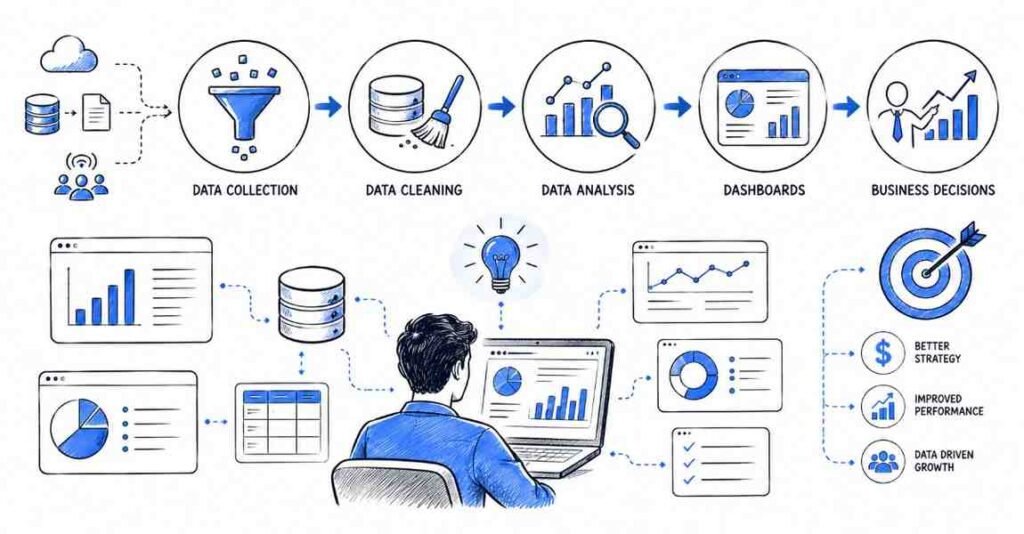
A data analytics professional collects, cleans, analyzes, and visualizes data to help businesses understand what is happening and what they should do next. The role is less about theory and more about solving practical business problems with numbers.
In simple terms, a data analytics professional helps teams answer questions like: What is selling well? Where are customers dropping off? Which campaign is working? What should we improve?
Main responsibilities
- Collect and clean data from different sources.
- Analyze trends and patterns.
- Build reports and dashboards.
- Write SQL queries to extract data.
- Use Excel and Python for analysis.
- Present findings to business teams.
- Support decision making with clear insights.
🚀 Kickstart Your Data Analytics Career
Join Our Data Analytics Course Today!
Why Data Analytics Is a Smart Career
Data analytics is a smart career because almost every company now depends on data to grow. Whether the business is in e-commerce, finance, healthcare, education, or marketing, it needs people who can turn information into decisions.
The field also offers a practical entry path. You do not need to be a computer science expert to start, and many learners can enter through Excel, SQL, and dashboard skills before moving into advanced analytics.
Why students choose it
- Strong demand across industries.
- Good mix of technical and business work.
- Useful for freshers and career switchers.
- Strong freelancing and remote opportunities.
- Easy to build a portfolio with real projects.
Data Analytics Roles Compared
Data analytics has several related job paths. Each one focuses on a different layer of analysis and reporting.
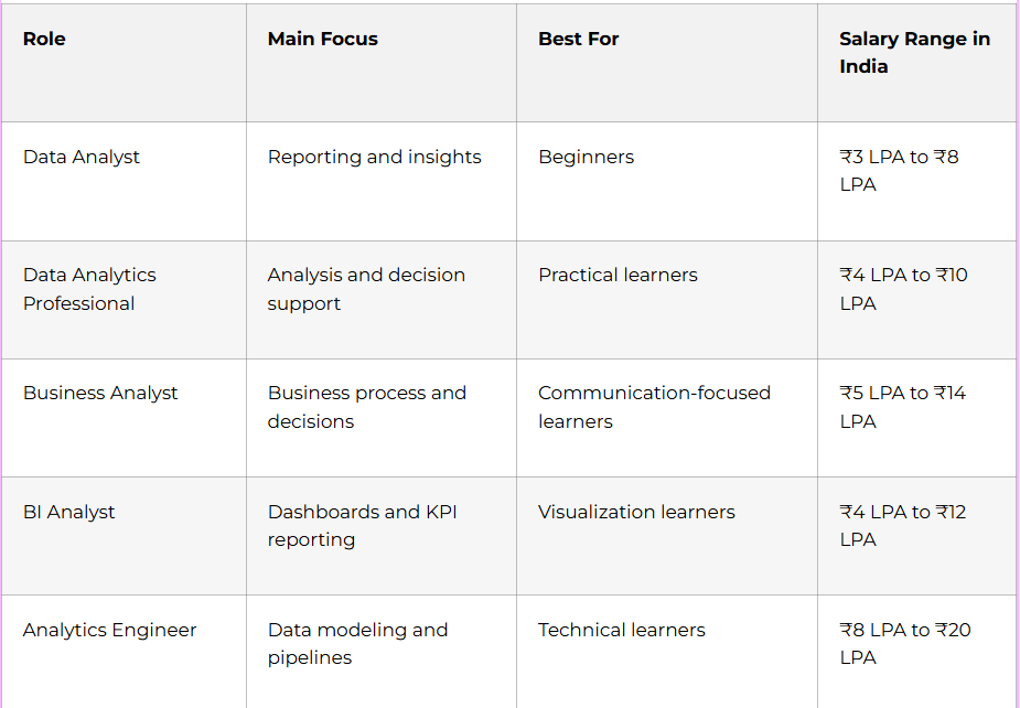
If you are starting out, a data analytics path is a strong choice because it gives you useful skills quickly and opens multiple job options.
Complete Learning Roadmap
Phase 1: Analytics Foundations
Before learning tools, you need to understand how data supports business decisions. This foundation helps you think like an analyst.
Focus on:
- What data analytics means.
- Types of data.
- Business metrics and KPIs.
- Problem solving with data.
- Basic statistics.
- Data quality and data validation.
- Reporting logic.
Phase 2: Excel and Spreadsheet Skills
Excel is still one of the most important tools in analytics. Many companies use it every day for reporting, tracking, and analysis.
Learn:
- Sorting and filtering.
- Basic formulas.
- Logical formulas like IF.
- Lookup formulas.
- Pivot tables.
- Charts and graphs.
- Conditional formatting.
- Data cleaning shortcuts.
Phase 3: SQL for Data Extraction
SQL is the language you use to pull data from databases. If you want to become a strong analytics professional, SQL is non-negotiable.
Learn:
- SELECT, WHERE, ORDER BY.
- GROUP BY and HAVING.
- JOINs.
- Subqueries.
- Aggregate functions.
- Window functions.
- Data filtering and segmentation.
Phase 4: Python for Analytics
Python helps you analyze larger datasets, automate tasks, and perform advanced data work. It is one of the most valuable skills in modern analytics.
Learn:
- Python basics.
- Data types and structures.
- Pandas for data analysis.
- NumPy for numerical work.
- Matplotlib and Seaborn for visualization.
- Jupyter Notebook.
- Data cleaning and transformation.
Phase 5: Dashboards and Visualization
Analytics is useful only when insights are easy to understand. Dashboards and visuals help managers see patterns quickly.
Learn:
- Bar charts, line charts, and pie charts.
- KPI dashboards.
- Power BI or Tableau basics.
- Filters and slicers.
- Storytelling with data.
- Presenting insights clearly.
Phase 6: Business Analysis and Reporting
A strong analytics professional also understands the business context behind the numbers. This is what helps you move from reporting to decision support.
Learn:
- Requirement gathering.
- Stakeholder communication.
- Reporting formats.
- Root cause analysis.
- Trend analysis.
- Business recommendations.
- Presentation skills.
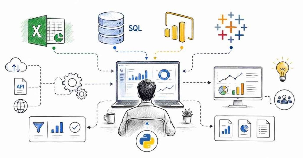
Excel, SQL, and Python
These three skills form the core of a data analytics career.
Excel skills to master
- Query writing.
- Joins and aggregations.
- Subqueries.
- Filtering and grouping.
- Analytical queries.
- Business reporting.
SQL skills to master
- Page structure planning.
- Information hierarchy.
- Navigation flow.
- Content placement.
- Layout variation testing.
Python skills to master
- Data cleaning.
- Data analysis.
- Visualization.
- Automation.
- Working with CSV and Excel files.
- Notebook-based reporting.
Salary Expectations in India
Salary depends on your portfolio quality, tool knowledge, and how well you explain design decisions. Designers with research, product thinking, and strong case studies usually grow faster.
Experience Level | Typical Salary |
Fresher | ₹3.5 LPA to ₹6 LPA |
1–3 years | ₹6 LPA to ₹12 LPA |
3–5 years | ₹12 LPA to ₹18 LPA |
5+ years | ₹18 LPA to ₹30 LPA+ |
Portfolio That Gets Interviews
A strong portfolio is the best way to prove that you can work with real data. Recruiters want to see practical examples, not just certificates.
What to include
- Excel dashboard project.
- SQL case study.
- Python data analysis notebook.
- Business insights report.
- KPI dashboard.
- Data cleaning example.
- Case study with clear recommendations.
Portfolio checklist
- Show the business question clearly.
- Include charts and tables.
- Explain the tools used.
- Add insights and recommendations.
- Keep files easy to understand.
- Use real-world sample datasets when possibl
Job Search Strategy
Your resume should highlight the tools and work styles that analytics employers value. The best resumes show both technical ability and business understanding.
Resume keywords
- Data analytics
- Excel
- SQL
- Python
- Dashboards
- Reporting
- Data visualization
- Business insights
- KPI tracking
- Power BI
- Tableau
- Data cleaning
Where to apply
- LinkedIn Jobs
- Naukri
- Indeed
- company career pages
- analytics job boards
- startup roles
- business support roles
Interview preparation
🎯 Prepare Smarter — Get 120+ Data Analytics Interview Questions & Answers
Be ready to answer questions like:
- How do you clean and prepare data?
- How do you write SQL queries for analysis?
- How do you use Excel for reporting?
- How do you explain insights to non-technical people?
- How do you build a dashboard?
- What is the difference between a report and an insight?
30-Day Starter Plan
If you want to begin now, follow this simple plan.
Week 1
- Learn analytics basics.
- Review common business metrics.
- Practice Excel shortcuts.
- Start simple spreadsheet exercises.
Week 2
- Learn Excel formulas and pivot tables.
- Practice data cleaning.
- Create one small dashboard.
- Analyze sample data.
Week 3
- Learn SQL basics.
- Practice joins and aggregations.
- Write queries on a sample database.
- Summarize results in a report..
Week 4
- Learn Python basics.
- Build a simple analysis notebook.
- Create a portfolio project.
- Update your resume and LinkedIn.
🧭 New to Analytics? Follow Our Step-by-Step Data Analytics Roadmap →

Why Learn Data Analytics at Frontlines Edutech
Frontlines Edutech is a practical choice for students and working professionals who want structured learning, regional support, and career-focused training. The best programs combine Excel, SQL, Python, dashboards, and project work in a way that makes job readiness realistic
What to look for in training
- Strong Excel and SQL foundation.
- Python analytics practice.
- Dashboard and reporting projects.
- Business analysis guidance.
- Resume and interview support.
- Regional-language explanation if needed.
Frequently Asked Questions
1. How long does it take to become a data analytics professional?
It usually takes 3 to 6 months of consistent learning to become job-ready, depending on your background and how much practical project work you do.
2. Is data analytics a good career in India?
Yes, it is a strong career because every company needs people who can understand data and support decisions. It is especially good for freshers and career switchers.
3. Which skill should I learn first?
Start with Excel, then move into SQL and Python. After that, learn dashboards and business analysis.
4. Do I need coding to become a data analytics professional?
You do not need advanced coding to start, but basic Python helps a lot. Excel and SQL are usually enough to begin your analytics journey.
5. What is the best specialization for beginners?
Data analyst and reporting roles are the easiest starting points. After that, you can move into BI, business analysis, or analytics engineering.
6. Can I get a job without experience?
Yes, if you have practical projects, a clean resume, and basic tool knowledge. Internships and portfolio work can help you enter the field faster.
7. Which tools should I learn first?
Start with Excel, SQL, Python, Power BI, and basic visualization tools. These cover the most common entry-level analytics tasks.
8. Is data analytics remote-friendly?
Yes, many analytics roles are remote-friendly because the work is digital and can be done with standard data tools and collaboration platforms.
9. What kind of projects should I show in interviews?
Show dashboards, SQL case studies, Excel reports, and Python analysis notebooks. Employers want to see that you can turn data into useful business insights.