How to Become a Traditional Data Scientist in 2026: Complete Career Guide
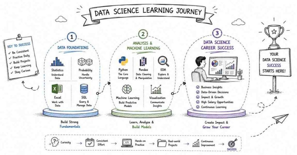
Table of Contents
Traditional data scientists are the people who turn raw business data into decisions, predictions, and measurable results, which is why the role stays valuable across industries. If you can work with Python, SQL, statistics, machine learning, and business thinking, you can build a strong and future-proof career in India. This guide will show you the exact roadmap to become job-ready in 2026, whether you are a fresher, an analyst, or a working professional moving into data science.
What a Traditional Data Scientist Does
A traditional data scientist studies data, finds patterns, builds predictive models, and explains what the numbers mean for a business. The job sits at the intersection of statistics, programming, and domain understanding.
Unlike pure software roles, data science is not only about writing code. It is about asking the right questions, cleaning messy data, testing hypotheses, and using machine learning where it actually adds value.
Main responsibilities
- Collect and clean data from multiple sources.
- Perform exploratory data analysis.
- Build statistical and machine learning models.
- Evaluate model performance and business usefulness.
- Communicate insights to stakeholders.
- Work with product, analytics, and engineering teams.
- Support forecasting, segmentation, churn analysis, and experimentation.
Why Traditional Data Science Is a Smart Career
Traditional data science remains a strong career because businesses still need people who can interpret data and make decisions from it. Even with newer AI tools, companies need professionals who understand data quality, statistical reasoning, and model evaluation.
This field also rewards structured learners. If you like math, logic, problem-solving, and practical coding, data science can become a high-value career path.
Why students choose it
- Strong demand in IT, fintech, retail, healthcare, and education.
- Good growth potential for analysts and engineers.
- Skills are useful across many industries.
- Portfolio work can open interview opportunities.
- Can lead to roles in analytics, ML, and product science.
Traditional Data Science Roles Compared
Traditional data science has several connected paths. Each role uses data differently, but the core foundation is similar.
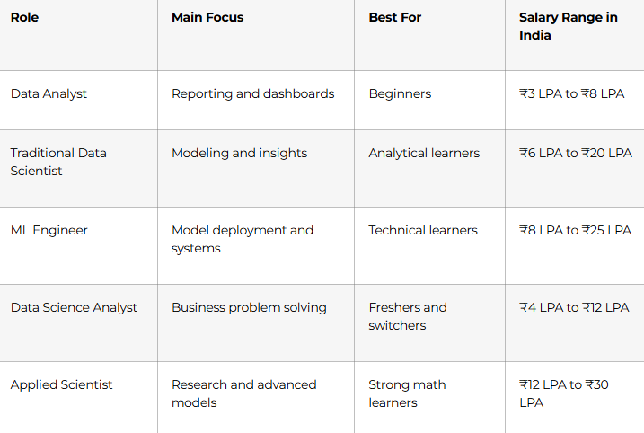
If you are starting out, a traditional data scientist path is usually best when you want a balanced combination of coding, statistics, and business problem solving.
Discover Your Data Scientist Career →
Complete Learning Roadmap
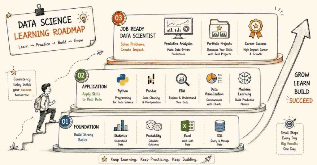
Phase 1: Data Foundations
Before learning machine learning, build a strong base in math, statistics, and data handling. This is the part that makes your thinking sharper.
Focus on:
- Descriptive statistics.
- Probability basics.
- Distributions.
- Hypothesis testing.
- Correlation and causation.
- Data cleaning fundamentals.
- Excel and spreadsheet logic.
Phase 2: Python for Data Science
Python is the most practical language for data science work. You do not need to master all of Python before starting, but you do need to be comfortable with the core tools.
Learn:
- Python syntax and data types.
- Lists, dictionaries, loops, and functions.
- NumPy for numerical operations.
- Pandas for data manipulation.
- Matplotlib and Seaborn for visualization.
- Jupyter Notebook for analysis.
Phase 3: SQL and Data Extraction
Most data science projects depend on data that lives in databases. That is why SQL is non-negotiable.
Learn:
- SELECT, WHERE, GROUP BY, ORDER BY.
- JOINs.
- Subqueries.
- Window functions.
- Aggregate functions.
- Basic query optimization.
- Reading data from relational databases.
Phase 4: Exploratory Data Analysis
EDA is where you learn what the data is actually saying. It helps you detect missing values, outliers, trends, and hidden relationships.
Learn to:
- Identify missing and duplicate data.
- Study distributions.
- Compare categories.
- Find correlations.
- Detect anomalies.
- Build clean charts and summary tables.
Phase 5: Machine Learning
Once your foundation is strong, move into machine learning. This is where you start building predictive systems.
Learn:
- Regression.
- Classification.
- Clustering.
- Decision trees.
- Random forests.
- XGBoost basics.
- Feature engineering.
- Train-test split.
- Overfitting and underfitting.
- Cross-validation.
Phase 6: Model Evaluation
A model is only useful if it performs well. You must know how to judge whether a model is actually solving the problem.
Learn:
- Accuracy, precision, recall, and F1 score.
- Confusion matrix.
- ROC-AUC.
- Mean squared error and MAE.
- Bias-variance tradeoff.
- Model tuning basics.
- Error analysis.
Follow the Data Scientist Roadmap →
Python, SQL, and Statistics
These three skills are the real base of a traditional data scientist.
Python skills to master
- Data cleaning and preprocessing.
- Dataframe operations.
- Visualization.
- Basic automation.
- Notebook-based analysis.
- Model building with scikit-learn.
SQL skills to master
- Querying large tables.
- Joining data sources.
- Segmenting customers.
- Preparing datasets for analysis.
- Writing reusable analytical queries.
Statistics skills to master
- Mean, median, mode.
- Variance and standard deviation.
- Probability concepts.
- Sampling methods.
- Confidence intervals.
- Hypothesis testing.
- A/B testing basics.
Salary Expectations in India
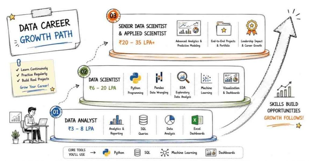
Salary depends on your math strength, project quality, communication skill, and how well you explain business value. Traditional data scientists usually earn more than basic reporting roles and can move into stronger roles with experience.
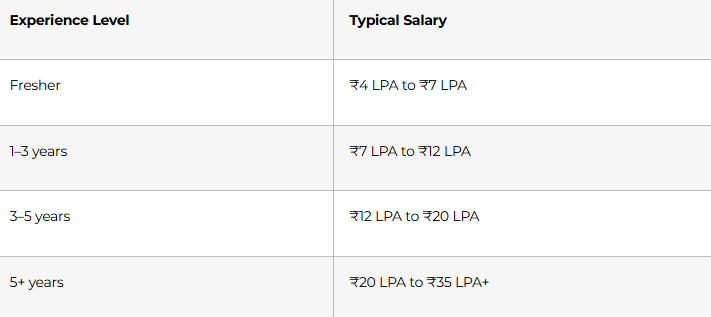
Professionals who understand both statistics and business context usually grow faster. Product companies and analytics-heavy firms often pay more than general support teams.
Practice Data Scientist Interview Questions →
Portfolio That Gets Interviews
A strong portfolio is the easiest way to prove you can handle real data science work. Your portfolio should show business problem solving, not just notebook code.
What to include
- One EDA project.
- One regression project.
- One classification project.
- One clustering or segmentation project.
- One SQL case study.
- One business dashboard or storytelling project.
- GitHub repository with clean README files.
Portfolio checklist
- Explain the business problem clearly.
- Show how you cleaned the data.
- Mention tools and libraries used.
- Include charts, metrics, and conclusions.
- Add limitations and next steps.
- Keep code organized and readable.
Job Search Strategy
Your resume and LinkedIn profile should make it obvious that you can work with data, not just talk about it.
Resume keywords
- Python
- SQL
- Statistics
- Machine learning
- Data analysis
- Pandas
- NumPy
- Scikit-learn
- Data visualization
- EDA
- A/B testing
- Feature engineering
Where to apply
- LinkedIn Jobs
- Naukri
- Indeed
- analytics and data job boards
- startup career pages
- internship portals
Interview preparation
Be ready to answer questions like:
- What is the difference between supervised and unsupervised learning?
- How do you handle missing values?
- What is overfitting?
- How do you choose evaluation metrics?
- How would you explain a model to a business team?
- How do you write an SQL query for analysis?
30-Day Starter Plan
If you want to start now, use this simple plan.
Week 1
- Learn basic Python syntax.
- Review statistics fundamentals.
- Install Jupyter Notebook.
- Create your first notebook.
Week 2
- Learn Pandas and NumPy.
- Practice data cleaning.
- Create simple charts.
- Explore one public dataset.
Week 3
- Learn SQL basics.
- Practice joins and aggregations.
- Write analytical queries.
- Start one EDA project.
Week 4
- Learn one machine learning algorithm.
- Build one simple prediction model.
- Write a project summary.
- Update your resume and LinkedIn.
Why Learn Data Science at Frontlines Edutech
Frontlines Edutech is a practical option for students and working professionals who want structured learning, regional support, and career-focused guidance. The best programs combine theory, coding, statistics, projects, and interview preparation.
What to look for in training
- Strong Python and SQL foundation.
- Statistics taught in a simple way.
- Real data projects.
- Model evaluation practice.
- Resume and interview support.
- Regional-language explanations if needed.
Frequently Asked Questions
Q1.How long does it take to become a traditional data scientist?
A.It usually takes 4 to 8 months of consistent learning to become job-ready, depending on your background and how much project work you complete.
Q2.Is traditional data science a good career in India?
A.Yes, it is a strong career because companies in every industry need data-driven decisions. It is especially good for learners who enjoy math, coding, and analysis.
Q3.Which skill should I learn first?
A.Start with Python, SQL, and statistics. Those three skills form the base for everything else in data science.
Q4.Do I need advanced math to become a data scientist?
A.You need a solid understanding of statistics and probability, but you do not need to be a pure mathematician. Practical problem solving matters more than advanced theory alone.
Q5.What is the best specialization for beginners?
A.A traditional data science path is ideal if you want to learn analysis, modeling, and business problem solving together. If you prefer dashboards and reporting, start with data analytics first.
Q6.Can I get a job without experience?
A.Yes, if you have practical projects, a strong resume, and clear fundamentals. Internships, Kaggle-style projects, and GitHub case studies can help a lot.
Q7.Which tools should I learn first?
A.Start with Python, Jupyter Notebook, Pandas, SQL, Matplotlib, and Scikit-learn. These cover most beginner-level data science tasks.
Q8.Is data science remote-friendly?
A.Yes, many data science roles are remote-friendly because the work is digital and collaborative. Strong communication and documentation skills help.
Q9.What kind of projects should I show in interviews?
A.Show EDA projects, prediction models, SQL case studies, and data storytelling work. Employers want to see that you can solve real problems with data.