Machine Learning Interview Preparation Guide

1. 300+ Technical Interview Questions & Answers
- Python Programming Fundamentals: 30 Questions
- Mathematics for Machine Learning: 30 Questions
- Data Libraries – NumPy: 35 Questions
- Data Libraries – Pandas: 25 Questions
- Data Visualization with Matplotlib: 15 Questions
- Machine Learning Fundamentals: 20 Questions
- Classification Models: 20 Questions
- Regression Models: 25 Questions
- Support Vector Machines: 30 Questions
- Decision Trees: 15 Questions
- Random Forests and Ensemble Methods: 40 Questions
- Unsupervised Learning Techniques: 15 Questions
- Neural Networks with Keras: 25 Questions
- Training Deep Neural Networks: 25 Questions
- TensorFlow Data Processing: 25 Questions
- Generative AI and LLMs: 25 Questions
⚡ Become a Job-Ready ML & Deep Learning Engineer — Join the Course Today!
Chapter 1: Python Programming Fundamentals
1.1 Basic Python Syntax and Data Types
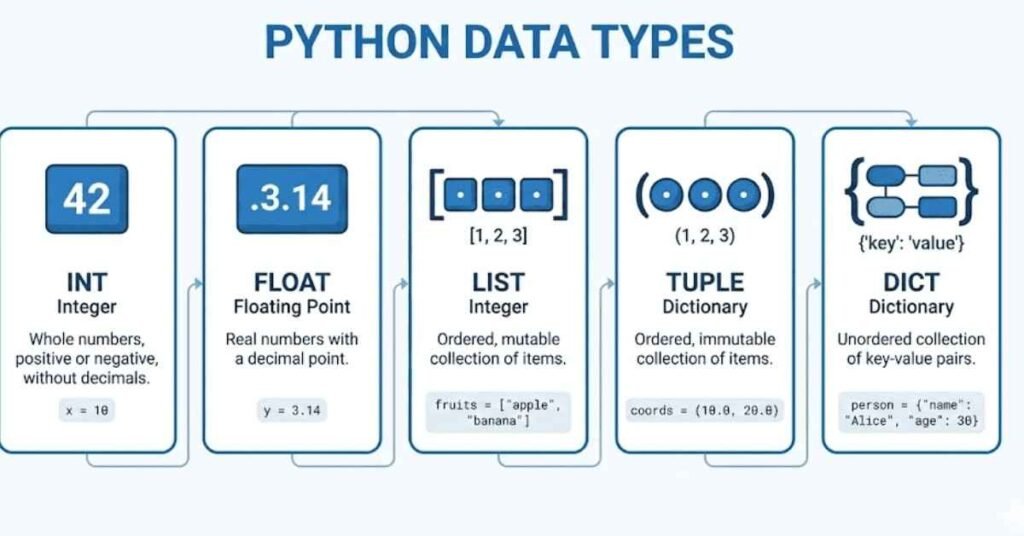
Q1. What are the main data types in Python used for machine learning?
Python has several core data types that you’ll use constantly in machine learning projects. The basic ones include integers for whole numbers, floats for decimal numbers, strings for text data, and booleans for true or false values. For machine learning specifically, you’ll work heavily with lists to store collections of data, tuples for immutable sequences, dictionaries for key-value pairs like feature names and values, and sets for unique elements. Understanding these is crucial because your entire dataset manipulation depends on handling these types correctly.
Q2. How do you handle string manipulation in Python for text preprocessing?
String manipulation is essential when working with text data in machine learning. You can use methods like split to break text into words, strip to remove whitespace, lower or upper to standardize case, and replace to substitute characters. For example, if you’re cleaning customer reviews, you might use text.lower().strip() to make everything lowercase and remove extra spaces. You can also use slicing with brackets to extract parts of strings, and the join method to combine multiple strings together.
Q3. What is the difference between a list and a tuple in Python?
Lists and tuples might look similar, but they have one key difference. Lists are mutable, meaning you can change them after creation by adding, removing, or modifying elements. Tuples are immutable, so once you create them, they cannot be changed. In machine learning, you use lists when you need flexibility, like storing training data that might be updated. Tuples are better for fixed data like image dimensions or coordinates that should never change. Tuples are also slightly faster and use less memory.
Q4. Explain list comprehension and why it’s useful in data processing.
List comprehension is a compact way to create lists in Python using a single line of code. Instead of writing a for loop with multiple lines, you can write something like squared_numbers equals bracket x multiplied by x for x in range ten bracket. This creates a list of squared numbers from zero to nine. In machine learning, list comprehension makes your code cleaner and often faster when transforming data, filtering datasets, or applying functions to multiple elements. It’s particularly useful when preprocessing features or creating new variables from existing ones.
Q5. What are Python dictionaries and how are they used in machine learning?
Dictionaries store data as key-value pairs, like a real dictionary stores words and definitions. In machine learning, dictionaries are incredibly useful for storing model parameters, hyperparameters, or mapping categorical values to numbers. For example, you might create a dictionary to map color names to numeric codes like red colon one, blue colon two. You can access values quickly using keys, add new pairs easily, and iterate through both keys and values. They’re also perfect for storing model configurations or evaluation metrics.
1.2 Control Flow and Loops
Q6. How do if-else statements work in Python and their role in ML pipelines?
If-else statements help your program make decisions based on conditions. In machine learning, you use them constantly for data validation, error handling, and implementing logic. For example, you might check if a value is missing before processing it, or decide which algorithm to use based on dataset size. The syntax is straightforward with if condition followed by colon, then indented code. You can add elif for multiple conditions and else for the default case. This conditional logic is fundamental for building robust ML pipelines.
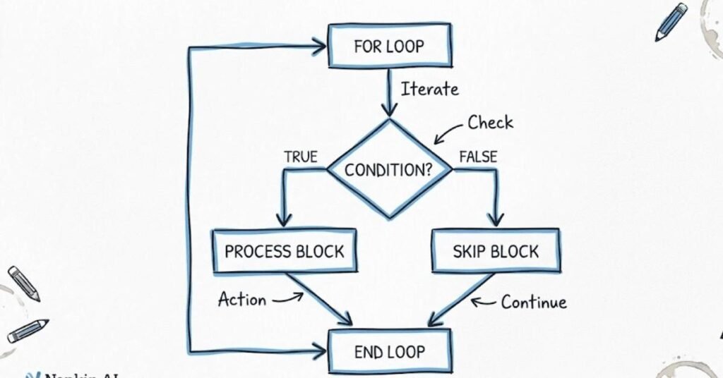
Q7. Explain the difference between for loops and while loops.
For loops iterate over a sequence for a predetermined number of times, while while loops continue until a condition becomes false. In machine learning, for loops are more common because you usually know how many iterations you need, like looping through each data point or each training epoch. You write for item in collection followed by your code. While loops are useful when you don’t know how many iterations you need upfront, like training a model until it reaches a certain accuracy threshold. Understanding when to use each makes your code more efficient.
Q8. What is the enumerate function and when should you use it?
Enumerate is a handy function that gives you both the index and the value when looping through a sequence. Instead of writing a counter variable manually, enumerate does it automatically. For example, for index comma value in enumerate my list gives you both. In machine learning, this is useful when you need to track position while processing data, like labeling which row you’re on in a dataset or tracking which epoch you’re in during model training. It makes your code cleaner and more readable.
Q9. How do you use break and continue statements in loops?
Break and continue give you control over loop execution. Break immediately exits the entire loop, while continue skips the rest of the current iteration and moves to the next one. In machine learning, you might use break when you’ve found what you’re looking for and don’t need to continue searching, saving computation time. Continue is useful for skipping invalid data points without stopping the entire process. For example, if you encounter a corrupted image in your dataset, you can use continue to skip it and process the next one.
Q10. What are nested loops and when are they necessary in ML?
Nested loops are loops inside other loops. They’re necessary when working with multidimensional data like matrices or images. For instance, to process every pixel in an image, you need one loop for rows and another for columns. In machine learning, you use nested loops for tasks like calculating distances between all pairs of points, comparing every prediction with every actual value, or performing grid search over multiple hyperparameters. However, they can be slow, so you should use vectorized operations when possible.
1.3 Functions and Lambda Expressions
Q11. Why are functions important in machine learning code?
Functions are reusable blocks of code that perform specific tasks. In machine learning, they help you organize code, avoid repetition, and make your work more maintainable. You might create a function for data preprocessing, another for model training, and another for evaluation. This way, you can call these functions whenever needed without rewriting code. Functions also make debugging easier because you can test each part independently. Good function design is the difference between messy scripts and professional ML code.
Q12. How do you define a function with default parameters?
Default parameters give function arguments preset values that are used if no value is provided when calling the function. You define them in the function signature like def train_model learning_rate equals zero point zero one. This is extremely useful in machine learning for setting default hyperparameters. Users can call your function with just required arguments and get sensible defaults, or they can override any parameter they want to customize. It makes your functions more flexible and user-friendly.
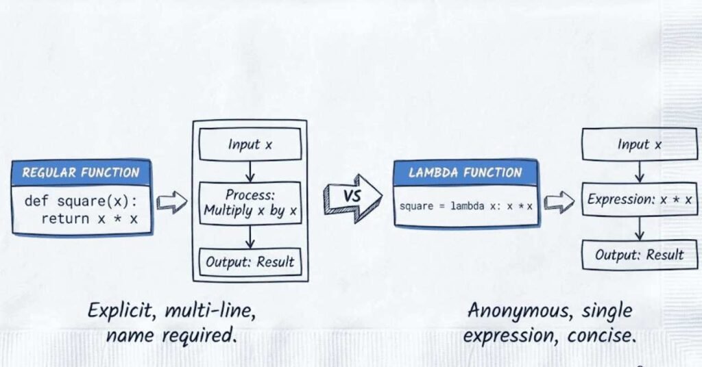
Q13. What are lambda functions and when should you use them?
Lambda functions are small anonymous functions defined in a single line without a formal def statement. They’re written as lambda arguments colon expression. In machine learning, you use them for quick operations that don’t need a full function definition, like applying a transformation to data. For example, when using map or filter functions, or sorting data with custom criteria. If your operation is simple and used only once, lambda is perfect. For complex operations used multiple times, regular functions are better.
Q14. Explain the concept of function scope and global variables.
Scope determines where variables can be accessed in your code. Variables defined inside a function have local scope and cannot be accessed outside. Variables defined at the top level have global scope and can be accessed anywhere. In machine learning projects, managing scope properly prevents bugs and makes code predictable. You should avoid global variables for model parameters or data because they can be accidentally modified. Instead, pass data as function arguments and return results explicitly.
Q15. How do you return multiple values from a function?
Python functions can return multiple values by separating them with commas. The function actually returns a tuple containing all values. For example, return accuracy comma loss comma model returns three values that you can unpack when calling the function. In machine learning, this is incredibly useful for returning multiple metrics from evaluation functions, or returning both predictions and confidence scores. You can unpack them as accuracy comma loss comma model equals evaluate_model or keep them as a tuple.
1.4 Object-Oriented Programming Concepts
Q16. What is Object-Oriented Programming and why is it used in ML frameworks?
Object-Oriented Programming organizes code around objects that combine data and functions that work with that data. Instead of having separate variables and functions floating around, you group related things together in classes. In machine learning, frameworks like TensorFlow and PyTorch use OOP extensively. Your model is an object with attributes like weights and methods like fit and predict. This makes code more organized, reusable, and easier to understand. You can create custom classes for datasets, models, or preprocessing pipelines.
Q17. How do you create a class in Python?
You create a class using the class keyword followed by the class name. Inside, you define an init method that runs when creating new objects, setting up initial attributes. Then you add other methods for different functionalities. For example, a NeuralNetwork class might have init to set layers, a forward method to make predictions, and a train method to update weights. Each method’s first parameter is self, which refers to the specific object instance. Classes help you build custom ML components that integrate smoothly with existing frameworks.
Q18. What is the difference between a class and an object?
A class is a blueprint or template that defines what something should look like and what it can do. An object is an actual instance created from that class. Think of a class as a cookie cutter and objects as the actual cookies made from it. In machine learning, you might have a DecisionTree class that defines how decision trees work. Then you create multiple tree objects from that class, each potentially trained on different data. The class defines the structure, while objects are the real working models.
Q19. Explain inheritance and how it’s used in ML model development.
Inheritance allows you to create new classes based on existing ones, inheriting their attributes and methods. The new class can add or override functionality. In machine learning, this is powerful for building model hierarchies. For example, Keras has a base Model class, and specific architectures like Sequential inherit from it. You can create your own custom model class that inherits from a base class, automatically getting standard methods while adding your specific logic. This promotes code reuse and consistency.
Q20. What are class attributes versus instance attributes?
Class attributes are shared by all instances of a class, while instance attributes are unique to each object. Class attributes are defined directly in the class body, while instance attributes are typically set in the init method using self. In machine learning, you might use a class attribute to store the algorithm name that all instances share, while instance attributes store the specific weights and hyperparameters unique to each trained model. Understanding this distinction prevents bugs where you accidentally share data between different models.
1.5 File Handling and Exception Management
Q21. How do you read data from a CSV file in Python?
Reading CSV files is a fundamental skill in machine learning since most datasets come in this format. You can use Python’s built-in csv module or the more powerful pandas library. With pandas, you simply write pd dot read_csv followed by the filename. This loads the entire dataset into a DataFrame that you can easily manipulate. You can specify parameters like which delimiter to use, whether there’s a header row, which columns to read, and how to handle missing values. Understanding these options helps you load data correctly.
Q22. What is the difference between reading a file with open versus using pandas?
Using open gives you raw file access where you read line by line and parse data yourself. This is useful for custom file formats or when you need fine control. Pandas read_csv, on the other hand, automatically parses the data into a structured DataFrame with rows and columns, handles different data types, and provides many options for data cleaning during import. For machine learning, pandas is usually better because it saves time and provides immediate access to powerful data manipulation methods. Use open for simple text files or custom formats.
Q23. How do you handle exceptions in Python and why is it important?
Exceptions are errors that occur during program execution. Handling them prevents your code from crashing unexpectedly. You use try-except blocks where you put potentially problematic code in the try section and handle errors in the except section. In machine learning, exceptions might occur when loading corrupted data files, when calculations produce invalid results like division by zero, or when memory runs out. Proper exception handling makes your ML pipelines robust, allowing them to skip bad data points or retry operations instead of failing completely.
Q24. What are the common exceptions you might encounter in ML code?
Several exceptions frequently appear in machine learning work. FileNotFoundError happens when trying to load a nonexistent dataset. ValueError occurs when functions receive the wrong type or shape of data, like passing strings to a function expecting numbers. MemoryError appears when your dataset is too large for available RAM. IndexError happens when accessing array indices that don’t exist. TypeError occurs when performing operations on incompatible types. KeyError appears when accessing missing dictionary keys. Knowing these helps you write better error handling code.
Q25. How do you write data to files in Python?
Writing data to files preserves your results for later use. With basic Python, you open a file in write mode and use the write method. For machine learning, you typically use pandas to write DataFrames to CSV files with to_csv, or numpy to save arrays with save or savetxt. You can also pickle Python objects to save entire models or preprocessors. When writing, consider whether to overwrite existing files or append to them, what format to use, and whether to compress large files. Proper file writing ensures reproducibility.
1.6 Python Libraries Overview
Q26. What are the essential Python libraries for machine learning?
Several libraries form the foundation of machine learning in Python. NumPy handles numerical arrays and mathematical operations efficiently. Pandas manages structured data in DataFrames, perfect for datasets with rows and columns. Matplotlib and Seaborn create visualizations to understand data and results. Scikit-learn provides standard machine learning algorithms and tools. TensorFlow and PyTorch enable deep learning. SciPy offers scientific computing functions. Each library has its strength, and professional ML engineers use combinations of these tools based on project needs.
Q27. Why is NumPy faster than regular Python lists for numerical operations?
NumPy arrays are much faster than Python lists for numerical work because of how they store data in memory. Lists store pointers to objects scattered in memory, while NumPy arrays store data in continuous blocks. This allows NumPy to use optimized C code for operations and leverage CPU features for parallel processing. When you multiply a NumPy array by a number, it happens in one optimized operation. With lists, you’d loop through each element individually in slow Python code. For machine learning with millions of numbers, this speed difference is crucial.
Q28. What is the purpose of importing libraries with aliases?
Importing libraries with aliases gives them shorter names for convenience. You write import numpy as np or import pandas as pd. This saves typing and follows community conventions that make code recognizable to other developers. Everyone knows np refers to NumPy and pd to Pandas. Using standard aliases also makes your code more readable and maintainable. However, for your own custom modules, descriptive imports are better than obscure aliases.
Q29. How do you install external Python libraries?
You install libraries using package managers, primarily pip. From your command line or terminal, you type pip install followed by the library name, like pip install scikit-learn. For specific versions, you add equals signs and version numbers. Conda is another popular option, especially for managing dependencies in data science environments. You can also install multiple packages at once by listing them in a requirements text file and running pip install minus r requirements dot txt. Managing installations properly ensures reproducibility across different computers.
Q30. What are virtual environments and why should you use them?
Virtual environments are isolated Python installations that keep project dependencies separate. Without them, all projects share the same libraries, which causes conflicts when different projects need different versions. You create a virtual environment with venv or conda, activate it, then install project-specific packages. In machine learning, this is essential because different projects might need different TensorFlow versions or conflicting package requirements. Virtual environments ensure your project works consistently and doesn’t break when you update libraries for other work.
Quick Tip: Need Clear Guidance? Explore Machine Learning How-To Guide!
Chapter 2: Mathematics for Machine Learning

2.1 Linear Algebra Essentials
Q31. What is a vector and how is it used in machine learning?
A vector is an ordered list of numbers that represents a point in space or a direction. In machine learning, vectors are everywhere. Each data point in your dataset is a vector where each number represents a feature. For example, a house might be represented as a vector containing size, number of rooms, and age. Model parameters are also vectors. Operations on vectors like addition, scaling, and dot products form the mathematical foundation of how algorithms learn patterns from data.
Q32. Explain what a matrix is and its role in ML algorithms.
A matrix is a rectangular array of numbers arranged in rows and columns. Your entire dataset is typically stored as a matrix where each row is a data point and each column is a feature. In deep learning, matrices represent layers of neurons and the weights connecting them. Many ML operations involve matrix multiplication, which efficiently computes relationships between features and predictions. Understanding matrices is essential because most algorithms work by performing mathematical operations on these number grids.
Q33. What is the dot product and why is it important?
The dot product takes two vectors and produces a single number by multiplying corresponding elements and summing the results. It measures how much two vectors point in the same direction. In machine learning, dot products appear everywhere. Linear regression predictions are dot products between your input features and learned weights. Neural network layers use dot products to combine inputs. Similarity between data points is often measured using dot products. This simple operation underpins much of how models make predictions.
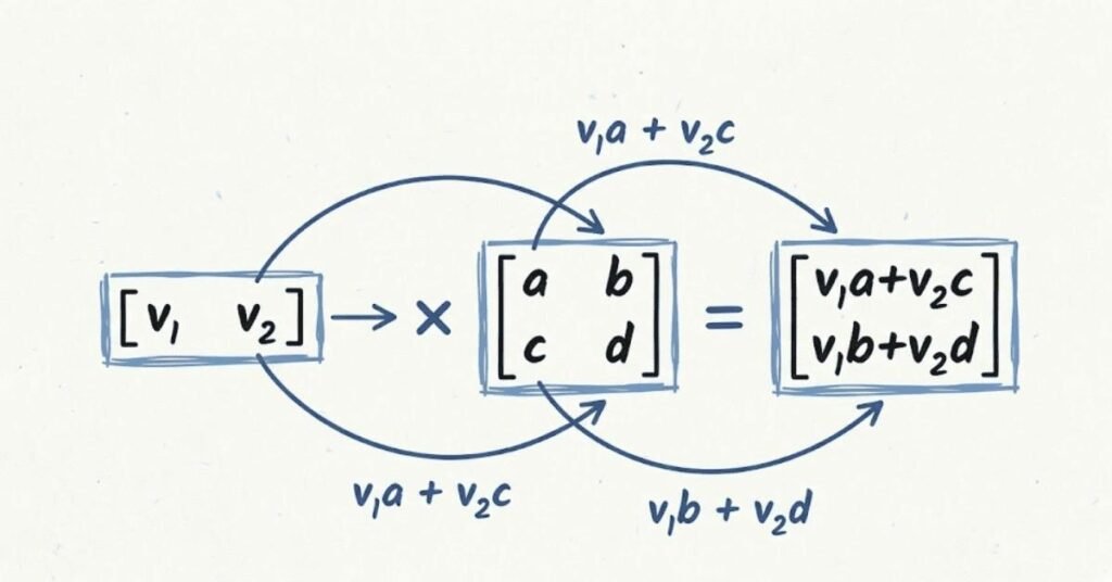
Q34. What does matrix multiplication represent in neural networks?
Matrix multiplication in neural networks represents information flowing through layers and being transformed. When you multiply your input matrix by a weight matrix, you’re computing a weighted sum for each neuron. Each neuron receives inputs from all previous neurons, multiplied by learned weights, and produces an output. This transformation happens at each layer. Understanding matrix multiplication helps you see how networks process information, why certain layer sizes work together, and how gradients flow backward during training.
Q35. What is the transpose of a matrix?
Transposing a matrix flips it over its diagonal, swapping rows and columns. A three by two matrix becomes a two by three matrix. In machine learning, transposition is used constantly in mathematical formulas. When computing gradients, you often need to transpose weight matrices. When reshaping data or preparing it for specific operations, transposition ensures dimensions align correctly. While it seems like a simple flip, proper transposition is crucial for making matrix operations work correctly in ML algorithms.
2.2 Matrix Operations and Transformations
Q36. What is the identity matrix and why is it special?
The identity matrix is a square matrix with ones on the diagonal and zeros elsewhere. It’s special because multiplying any matrix by the identity matrix leaves it unchanged, similar to how multiplying a number by one leaves it unchanged. In machine learning, the identity matrix appears in regularization techniques, in understanding inverse matrices, and in initialization strategies for neural networks. It represents the concept of doing nothing, which is sometimes exactly what you need mathematically.
Q37. Explain matrix inversion and when it’s used.
Matrix inversion finds a matrix that, when multiplied with the original, produces the identity matrix. It’s like finding the reciprocal of a number. In machine learning, inversion appears in the closed-form solution for linear regression and in certain optimization algorithms. However, computing inverses is expensive and numerically unstable, especially for large matrices. Modern ML typically avoids direct inversion, using iterative methods instead. Understanding inversion helps you grasp why some algorithms work and why others use different approaches.
Q38. What are eigenvalues and eigenvectors?
Eigenvalues and eigenvectors describe special directions in which a matrix stretches space. When you multiply a matrix by its eigenvector, the result points in the same direction, just scaled by the eigenvalue. These concepts appear in Principal Component Analysis, which finds directions of maximum variance in data. They also help analyze neural network stability and behavior. While the math can be complex, think of eigenvectors as important directions in your data and eigenvalues as how important each direction is.
Q39. What is matrix rank and why does it matter?
Matrix rank tells you how many independent rows or columns a matrix has. A matrix is full rank if all rows or columns are independent, meaning each provides unique information. In machine learning, rank matters for several reasons. Low rank matrices indicate redundant features in your data. Rank affects whether certain operations like inversion are possible. In dimensionality reduction, you deliberately create lower rank approximations of data. Understanding rank helps you identify data quality issues and choose appropriate algorithms.
Q40. How do you determine if a matrix is singular?
A singular matrix is one that cannot be inverted, similar to how you cannot divide by zero. You can identify singular matrices by calculating their determinant, which equals zero for singular matrices. Singular matrices occur when rows or columns are linearly dependent, meaning some can be expressed as combinations of others. In machine learning, singularity indicates problems like perfect multicollinearity in linear regression. Modern algorithms handle near-singular matrices using regularization techniques that add small values to make inversion stable.
2.3 Statistics Fundamentals
Q41. What is the difference between mean, median, and mode?
These three measures describe the center of your data differently. Mean is the average, calculated by summing all values and dividing by count. It’s sensitive to extreme values called outliers. Median is the middle value when data is sorted, making it robust to outliers. Mode is the most frequent value. In machine learning, choosing the right measure matters. For house prices with some mansions, median better represents typical prices than mean. For predicting categories, mode makes sense. Understanding these differences helps you summarize data appropriately.
Q42. Explain variance and standard deviation.
Variance measures how spread out your data is from the mean. You calculate it by finding the average squared difference from the mean. Standard deviation is simply the square root of variance, putting the measure back in the original units. In machine learning, these statistics appear everywhere. Feature scaling uses standard deviation. Understanding prediction uncertainty requires variance. High variance in model predictions indicates overfitting. Low variance might indicate underfitting. These measures help you understand both your data and model behavior.
Q43. What is covariance and correlation?
Covariance measures whether two variables tend to increase or decrease together. Positive covariance means they move together, negative means they move opposite, and zero means no relationship. Correlation is standardized covariance ranging from negative one to positive one, making it easier to interpret. In machine learning, correlation helps you understand relationships between features, identify redundant features, and interpret model behavior. High correlation between features might indicate multicollinearity problems in linear models.
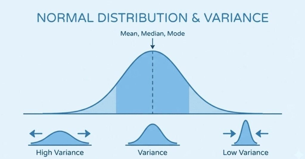
Q44. What is a normal distribution and why is it important?
A normal distribution, shaped like a bell curve, describes how many natural phenomena behave. Most values cluster around the mean, with fewer values appearing as you move away. It’s completely described by its mean and standard deviation. In machine learning, normal distributions appear constantly. Many algorithms assume data is normally distributed. Error terms in linear regression should be normally distributed. The Central Limit Theorem explains why averages tend toward normal distributions. Understanding normality helps you choose appropriate models and validate assumptions.
Q45. What are percentiles and quartiles?
Percentiles divide your data into hundred equal parts. The 25th percentile means twenty-five percent of data falls below that value. Quartiles are specific percentiles dividing data into four parts, at the 25th, 50th, and 75th percentiles. In machine learning, percentiles help you understand data distribution, identify outliers, and create features. The interquartile range between the 25th and 75th percentiles is robust to outliers. When analyzing model errors, looking at different percentiles reveals whether your model struggles with certain types of predictions.
2.4 Probability Theory
Q46. What is probability and how is it used in machine learning?
Probability quantifies uncertainty, ranging from zero for impossible events to one for certain events. In machine learning, probability is fundamental. Classification models output probability estimates for each class. Bayesian methods explicitly model uncertainty. Probabilistic graphical models represent relationships between variables. Understanding probability helps you interpret model confidence, quantify prediction uncertainty, and make better decisions when outcomes are uncertain. Many ML algorithms are essentially sophisticated probability calculators finding the most likely explanation for data.
Q47. Explain conditional probability.
Conditional probability measures the chance of one event happening given that another has occurred. Written as P of A given B, it represents the probability of A when you know B is true. In machine learning, conditional probabilities are everywhere. Naive Bayes classifiers compute the probability of a class given observed features. In sequence models, you predict the next word given previous words. Medical diagnosis models estimate disease probability given symptoms. Understanding conditional probability helps you build models that incorporate available information to make better predictions.
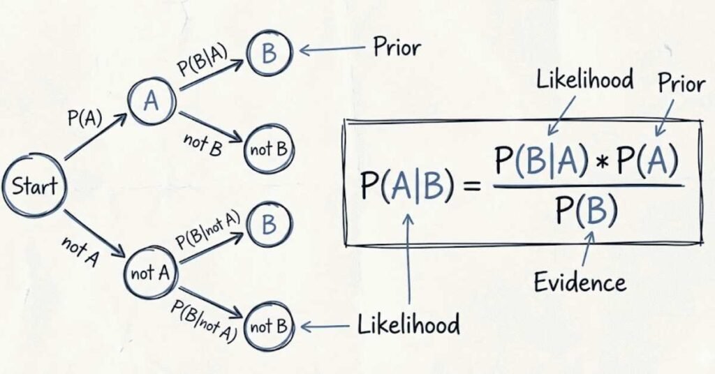
Q48. What is Bayes Theorem?
Bayes Theorem provides a formula for updating beliefs based on new evidence. It relates the probability of A given B to the probability of B given A. In machine learning, this enables you to reverse conditional probabilities. Given how likely symptoms are for each disease, Bayes Theorem computes how likely each disease is given observed symptoms. Naive Bayes classifiers use this principle. Bayesian optimization for hyperparameter tuning applies it. The theorem formalizes learning from data, making it foundational to many ML approaches.
Q49. What is the difference between independent and dependent events?
Independent events don’t affect each other. Knowing one happened doesn’t change the probability of the other. Coin flips are independent since previous results don’t influence future ones. Dependent events do affect each other. Drawing cards without replacement creates dependence since each draw changes remaining possibilities. In machine learning, assuming independence often simplifies calculations, like Naive Bayes assuming features are independent. Understanding when this assumption holds or fails affects model accuracy and choice of algorithm.
Q50. What are random variables?
A random variable assigns numbers to outcomes of random processes. Rather than describing outcomes as heads or tails, you assign numeric values like zero or one. Random variables can be discrete, taking specific values like integers, or continuous, taking any value in a range. In machine learning, your data can be viewed as observations of random variables. Features are random variables with certain distributions. Understanding this perspective helps you apply probability theory to data analysis and modeling.
2.5 Differential Calculus Applications
Q51. What is a derivative and why does it matter in machine learning?
A derivative measures how a function changes as its input changes, representing the slope at each point. In machine learning, derivatives are crucial for training models. Gradient descent uses derivatives to determine how to adjust model parameters to reduce error. The derivative tells you which direction to move parameters and how quickly the error changes. Without derivatives, you couldn’t efficiently optimize the millions of parameters in modern neural networks. Understanding derivatives helps you grasp how learning algorithms actually work.
Q52. What is a gradient?
A gradient is the multidimensional version of a derivative. While a derivative applies to functions with one input, gradients apply to functions with multiple inputs. The gradient is a vector pointing in the direction of steepest increase, with each component being the partial derivative with respect to one input. In machine learning, you compute gradients of your loss function with respect to all model parameters. These gradients tell you how to adjust each parameter to reduce error, forming the basis of gradient descent optimization.
Q53. Explain the chain rule and its importance in backpropagation.
The chain rule is a calculus technique for finding derivatives of composite functions. If you have a function inside another function, the chain rule tells you how to break down the derivative into manageable pieces. In neural networks, backpropagation uses the chain rule to compute gradients layer by layer, flowing backward from output to input. Each layer’s gradient depends on the next layer’s gradient, creating a chain of computations. Without the chain rule, training deep neural networks would be impossible since you couldn’t efficiently compute all the needed gradients.
Q54. What is a partial derivative?
A partial derivative measures how a function changes with respect to one variable while keeping all other variables constant. For a function with multiple inputs, you have one partial derivative for each input. In machine learning, when optimizing models with many parameters, you compute partial derivatives for each parameter. This tells you how changing just that parameter affects your loss. Collecting all partial derivatives gives you the gradient. Understanding partial derivatives helps you see how each parameter contributes to model performance.
Q55. What is the purpose of second derivatives in optimization?
Second derivatives measure how the rate of change itself changes, indicating curvature. While first derivatives give slope, second derivatives tell whether you’re in a valley, on a hill, or at an inflection point. In machine learning optimization, second derivatives appear in advanced methods like Newton’s method and in understanding convergence behavior. Positive second derivatives indicate you’re in a valley, suggesting you’ve found a minimum. Negative values indicate a hill or maximum. Second-order optimization methods use this curvature information to converge faster than simple gradient descent.
2.6 Mathematical Optimization Basics
Q56. What is an optimization problem in machine learning?
An optimization problem involves finding the best solution from all possible solutions according to some criterion. In machine learning, you optimize model parameters to minimize prediction error or maximize accuracy. The criterion you optimize is called the objective or loss function. The challenge is that with millions of parameters and complex models, finding the absolute best solution is often impossible. Instead, algorithms find good solutions using techniques like gradient descent. Understanding optimization helps you choose algorithms, set hyperparameters, and diagnose training issues.
Q57. What is a local minimum versus a global minimum?
A local minimum is a point where the function value is lower than nearby points but might not be the absolute lowest point overall. A global minimum is the absolute lowest point across the entire function. Imagine a hilly landscape where local minima are valleys surrounded by higher ground, while the global minimum is the deepest valley overall. In machine learning, optimization algorithms often get stuck in local minima, finding decent but not optimal solutions. Deep learning with many parameters has countless local minima, yet surprisingly, most are acceptably good for practical purposes.
Q58. What is a convex function and why is convexity important?
A convex function curves upward like a bowl, having the property that any local minimum is also the global minimum. Mathematically, the line segment between any two points on the function lies above the function itself. Convex functions are important in machine learning because they’re easier to optimize. If your loss function is convex, gradient descent is guaranteed to find the global minimum. Linear regression with squared error is convex. However, neural networks are non-convex, making optimization more challenging but still practically solvable.
Q59. What are constraints in optimization problems?
Constraints are restrictions on acceptable solutions. You might require parameters to be positive, sum to one, or stay within certain bounds. Constrained optimization finds the best solution while satisfying all constraints. In machine learning, constraints appear when normalizing probabilities, enforcing sparsity, or limiting model complexity. Some algorithms handle constraints directly, while others use penalty methods that add terms to the loss function when constraints are violated. Understanding constraints helps you formulate problems correctly and choose appropriate optimization methods.
Q60. What is the difference between convex and non-convex optimization?
Convex optimization deals with convex functions where every local minimum is global, making problems easier to solve with guarantees. Non-convex optimization tackles functions with multiple local minima and complex landscapes where finding the global minimum is hard or impossible. Traditional machine learning often uses convex optimization. Deep learning uses non-convex optimization since neural networks aren’t convex. Despite theoretical difficulties, practical algorithms and techniques like momentum, adaptive learning rates, and good initialization make non-convex optimization work remarkably well for training deep models.
Chapter 3: Data Libraries - NumPy

3.1 Introduction to NumPy Arrays
Q61. What is NumPy and why is it essential for machine learning?
NumPy is the fundamental package for numerical computing in Python, providing support for large multidimensional arrays and matrices along with mathematical functions. It’s essential for machine learning because it makes numerical operations fast and convenient. Instead of using slow Python loops, NumPy performs operations on entire arrays at once using optimized C code. All other ML libraries build on NumPy. Your data starts as NumPy arrays, matrices in scikit-learn are NumPy arrays, and even TensorFlow tensors work similarly to NumPy arrays.
Q62. What is the difference between a Python list and a NumPy array?
Python lists are flexible containers that can hold different types of objects, but they’re slow for numerical operations. NumPy arrays must contain elements of the same type, but this restriction enables massive speed improvements. Arrays store data in continuous memory blocks, allowing vectorized operations that process all elements simultaneously. For machine learning with thousands or millions of numbers, NumPy arrays are hundreds of times faster. Lists are for general collections, while arrays are for numerical computation where performance matters.
Q63. How do you create a NumPy array from a Python list?
Creating NumPy arrays from lists is straightforward. You use np.array and pass your list as an argument. For example, np.array bracket one comma two comma three creates a one-dimensional array. For two-dimensional arrays, you pass a list of lists where each inner list becomes a row. You can also specify the data type using the dtype parameter, controlling whether you want integers, floats, or other types. This conversion is often your first step when bringing data into NumPy for machine learning processing.
Q64. What are NumPy array attributes like shape, size, and dtype?
NumPy arrays have useful attributes that describe them. Shape is a tuple showing dimensions, like three comma four for a three-row, four-column matrix. Size gives the total number of elements. Dtype tells you the data type of elements, like int64 or float32. Ndim shows the number of dimensions. These attributes help you understand your data structure, debug dimension mismatches, and verify operations produce expected results. Checking shape is especially important to ensure arrays align correctly for mathematical operations.
Q65. How do you check and change the data type of a NumPy array?
You check data type using the dtype attribute. To change types, use the astype method with the desired type. For example, array.astype np.float32 converts to 32-bit floats. Type conversion matters in machine learning for memory efficiency and computational speed. Using float32 instead of float64 halves memory usage and often speeds up GPU computation without significantly affecting accuracy. Converting data types appropriately optimizes your pipeline while ensuring numerical precision meets your needs.
3.2 Array Creation and Manipulation
Q66. What are different ways to create NumPy arrays besides converting lists?
NumPy provides many convenience functions for array creation. np.zeros creates arrays filled with zeros, useful for initializing result containers. np.ones creates arrays of ones. np.arange creates sequences of numbers similar to Python’s range. np.linspace creates evenly spaced numbers between two endpoints. np.eye creates identity matrices. np.random provides functions for random arrays with various distributions. In machine learning, you use these for initializing weights, creating test data, generating ranges for plotting, and setting up computational structures.
Q67. How does np.arange differ from np.linspace?
np.arange and np.linspace both create sequences, but differently. np.arange takes a start, stop, and step size, creating values spaced by the step amount. However, the exact endpoint might not be included due to floating-point precision. np.linspace takes a start, stop, and number of points, creating exactly that many evenly spaced values including both endpoints. Use arange when you care about step size, like creating array indices. Use linspace when you care about having a specific number of points, like creating a smooth range for plotting model predictions.
Q68. What is broadcasting in NumPy?
Broadcasting is NumPy’s way of performing operations on arrays of different shapes without explicitly replicating data. When you add a small array to a large one, NumPy automatically broadcasts the small array across the large one. For example, adding a single number to an array adds that number to every element. Adding a one-dimensional array to a two-dimensional array can add the same vector to every row. Broadcasting eliminates loops, saves memory, and makes code cleaner. Understanding broadcasting rules helps you write efficient vectorized code.
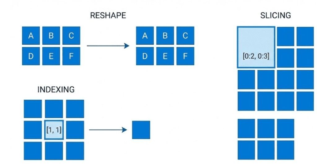
Q69. How do you reshape NumPy arrays?
Reshaping changes array dimensions without changing data. Use the reshape method with the desired shape. For example, array.reshape three comma four transforms a twelve-element array into a three-by-four matrix. The total number of elements must remain the same. You can use negative one in one dimension to have NumPy calculate that dimension automatically. In machine learning, reshaping is constant. You flatten images into vectors for some algorithms, reshape predictions to match targets, and adjust dimensions for specific operations. The reshape method is essential for preparing data correctly.
Q70. What does flattening an array mean?
Flattening converts a multidimensional array into a one-dimensional vector. You use the flatten or ravel methods. The difference is that flatten creates a copy while ravel creates a view when possible. In machine learning, flattening is common when feeding multidimensional data like images into algorithms expecting vectors. For example, a 28 by 28 pixel image becomes a 784-element vector. Understanding when to flatten and when to preserve structure is important for different algorithms and network architectures.
3.3 Indexing and Slicing Techniques
Q71. How does NumPy array indexing work?
NumPy indexing accesses specific elements or subsets of arrays. For one-dimensional arrays, use bracket notation with an index like array bracket three. For multidimensional arrays, separate indices with commas like array bracket two comma five for row two, column five. Negative indices count from the end. You can index multiple dimensions at once, making it easy to access specific values in matrices or higher-dimensional tensors. Proper indexing is fundamental for selecting data, examining specific values, and debugging your code.
Q72. Explain slicing in NumPy arrays.
Slicing extracts portions of arrays using colon notation. array bracket start colon stop colon step specifies the range. Omitting values uses defaults: start defaults to beginning, stop to end, and step to one. For multidimensional arrays, you slice each dimension separately with commas. For example, array bracket colon comma one selects all rows and column one. Slicing creates views rather than copies, meaning changes affect the original array. In machine learning, slicing selects training batches, extracts specific features, or focuses on particular data regions.
Q73. What is fancy indexing?
Fancy indexing uses arrays of indices to select elements in arbitrary order. Instead of simple slices, you pass an array of positions you want. For example, array bracket bracket zero comma two comma five bracket bracket selects elements at positions zero, two, and five. For multidimensional arrays, you can fancy index each dimension. This is powerful for selecting non-contiguous data, reordering elements, or picking specific samples from a dataset. Unlike slicing, fancy indexing creates copies rather than views.
Q74. How do you use boolean indexing?
Boolean indexing uses true-false arrays to select elements meeting certain conditions. You create a boolean array with a condition like array greater than five, which marks which elements satisfy the condition. Then you use this boolean array as an index like array bracket array greater than five bracket to select only those elements. In machine learning, boolean indexing filters data, removes outliers, selects specific classes, or masks invalid values. It’s an elegant way to work with subsets of data based on logical conditions.
Q75. What is the difference between a view and a copy?
A view references the original array’s data, so changes to the view affect the original. A copy is independent, so changes don’t affect the original. Slicing typically creates views, while fancy indexing creates copies. You can explicitly create copies with the copy method. This distinction matters in machine learning when you want to preserve original data while working with transformations. Accidentally modifying original data through a view causes subtle bugs. Understanding views versus copies prevents unexpected behavior and helps manage memory efficiently.
3.4 Array Transposition Methods
Q76. What does transposing an array mean?
Transposing swaps array dimensions, most commonly flipping a matrix’s rows and columns. You use the transpose method or the T attribute. An array with shape three by four becomes four by three. The element at row I, column J becomes the element at row J, column I. In machine learning, transposition aligns dimensions for matrix multiplication, prepares data for specific algorithms, and adjusts output formats. Understanding when to transpose prevents dimension errors and ensures operations work correctly.
Q77. How do you transpose multidimensional arrays?
For arrays with more than two dimensions, you specify how to permute axes using the transpose method with an axis argument. For example, transpose with argument zero comma two comma one swaps the second and third axes. This gives you complete control over dimension reordering. In deep learning, you might rearrange image tensors from channels-last to channels-first format or reorganize batch dimensions. The default transpose reverses all axes, but explicit axis specification lets you make precise rearrangements.
Q78. What is the swapaxes method?
The swapaxes method exchanges two specific axes while leaving others unchanged. You specify which two axes to swap. This is more convenient than full transposition when you only need to exchange two dimensions. For example, swapaxes one comma two swaps the second and third axes. In machine learning, this helps reformat tensors for different frameworks or operations. It’s particularly useful in image processing when you need to move the channel dimension to a different position.
Q79. When do you need to transpose arrays in ML workflows?
Transposition is needed frequently in machine learning. Matrix multiplication requires dimensions to align correctly, often necessitating transposition. Computing gradients involves transposing weight matrices. Some algorithms expect features as columns while your data has features as rows. Converting between different data format conventions requires transposition. Deep learning frameworks sometimes differ in whether they expect channels-first or channels-last image formats. Recognizing when dimensions don’t align and knowing how to transpose correctly is essential for preventing errors.
Q80. What is the moveaxis function?
The moveaxis function moves an axis from one position to another, sliding other axes to make room. You specify the source and destination positions. This provides another way to reorganize dimensions, sometimes more intuitive than transpose. For example, moveaxis source equals zero comma destination equals two moves the first axis to the third position. In machine learning, this helps rearrange tensors when you need a specific dimension order for operations or when converting between different data format conventions.
3.5 Universal Array Functions
Q81. What are universal functions in NumPy?
Universal functions, or ufuncs, are functions that operate element-wise on arrays, performing the same operation on each element efficiently. Examples include np.exp, np.log, np.sqrt, and trigonometric functions. These functions are implemented in compiled C code, making them much faster than Python loops. They also support broadcasting, allowing operations between arrays of different shapes. In machine learning, ufuncs appear everywhere: applying activation functions, computing losses, transforming features, and normalizing data. Understanding ufuncs helps you write fast, vectorized code.
Q82. How do mathematical operations work on NumPy arrays?
NumPy arrays support element-wise mathematical operations using standard operators. Addition, subtraction, multiplication, and division with the plus, minus, asterisk, and slash operators work element by element. Powers use the double asterisk operator. These operations are vectorized, applying to entire arrays at once without loops. For example, array times two multiplies every element by two. array1 plus array2 adds corresponding elements. This makes mathematical expressions clean and fast. Element-wise operations are default; for matrix multiplication, use the at symbol or dot method.
Q83. What is the difference between multiply and dot in NumPy?
The multiply function or asterisk operator performs element-wise multiplication, multiplying corresponding elements and returning an array of the same shape. The dot function or at symbol performs matrix multiplication following linear algebra rules, computing dot products of rows and columns. For two-dimensional arrays, dot performs traditional matrix multiplication. The shapes must be compatible: the inner dimensions must match. In machine learning, element-wise multiplication appears in scaling and masks, while dot multiplication computes predictions, propagates signals through networks, and performs many other core operations.
Q84. How do you apply functions like exponential or logarithm to arrays?
NumPy provides ufuncs for common mathematical functions. np.exp computes exponential for each element, used in softmax and sigmoid activations. np.log computes natural logarithm, appearing in cross-entropy loss. np.log10 and np.log2 provide other logarithm bases. np.sqrt computes square roots. These functions work element-wise on entire arrays, much faster than looping. For example, np.exp array exponentiates every element. These operations are fundamental in machine learning for transforming data, computing activations, and calculating metrics.
Q85. What are aggregation functions in NumPy?
Aggregation functions reduce arrays to single values or lower dimensions by computing statistics. np.sum adds elements, np.mean computes averages, np.max and np.min find extremes, np.std calculates standard deviation. You can aggregate the entire array or along specific axes. For example, np.mean array axis equals zero averages each column. In machine learning, aggregations compute batch statistics, calculate overall metrics, find maximum predictions, normalize features, and reduce dimensions. Understanding aggregation axes is crucial for operating on the correct dimensions of your data.
3.6 Array Processing Operations
Q86. How do you stack arrays together?
NumPy provides several stacking functions. np.vstack stacks arrays vertically, adding rows. np.hstack stacks horizontally, adding columns. np.concatenate joins arrays along an existing axis. np.stack creates a new axis and stacks along it. For example, stacking two arrays with shape ten by five vertically gives twenty by five. In machine learning, you stack arrays to combine datasets, merge batches, or assemble predictions. Choosing the right stacking function depends on how you want arrays arranged and whether you need a new dimension.
Q87. What is the difference between concatenate and stack?
Concatenate joins arrays along an existing axis, making that axis longer while keeping dimensions the same. Stack creates a new axis and arranges arrays along it, increasing dimensionality. For example, concatenating two ten by five arrays along axis zero gives twenty by five. Stacking them creates a two by ten by five array. In machine learning, concatenate combines similar data like adding more samples. Stack organizes separate arrays into a structured collection, useful when combining predictions from multiple models or organizing data batches.
Q88. How do you split arrays?
NumPy provides splitting functions opposite to stacking. np.split divides an array into multiple sub-arrays at specified positions. np.array_split splits into roughly equal parts even if the division isn’t exact. np.vsplit and np.hsplit split vertically and horizontally. For example, np.split array comma three splits into three equal parts along the first axis. In machine learning, splitting creates training and validation sets, separates features and targets, divides data into batches, or breaks large arrays into manageable chunks for processing.
Q89. What are tile and repeat functions?
The tile function repeats an entire array multiple times, like laying tiles. np.tile array comma two comma three repeats the array twice vertically and three times horizontally. The repeat function repeats individual elements. np.repeat array comma three repeats each element three times in place. In machine learning, these functions create replicated data for augmentation, broadcast values to match dimensions, or generate repeated patterns. Understanding when to use tile versus repeat depends on whether you want whole arrays duplicated or individual elements repeated.
Q90. How do you sort NumPy arrays?
NumPy provides sorting functions. np.sort returns a sorted copy, while array.sort sorts in place. You can sort along different axes for multidimensional arrays. np.argsort returns indices that would sort the array rather than sorted values themselves, useful for reordering other arrays consistently. np.partition partially sorts, efficiently finding top K elements without fully sorting. In machine learning, sorting identifies top predictions, ranks features by importance, orders data for visualization, or finds nearest neighbors. Choosing between sort and argsort depends on whether you need values or indices.
3.7 Array Input and Output Handling
Q91. How do you save NumPy arrays to files?
NumPy provides several saving functions. np.save writes a single array in binary format with npy extension. np.savez saves multiple arrays in a single compressed file with npz extension, accessing each array by name. For human-readable output, np.savetxt writes text files. Binary formats are faster and preserve precision perfectly but aren’t human-readable. In machine learning, saving arrays preserves processed datasets, stores model weights, saves predictions for analysis, or checkpoints intermediate results. Regular saving prevents data loss from crashes or errors.
Q92. How do you load NumPy arrays from files?
Loading matches saving functions. np.load reads npy files, returning the array. For npz files containing multiple arrays, np.load returns a dictionary-like object where you access arrays by name. np.loadtxt reads text files into arrays. When loading, verify the array shape and data type match expectations to catch corruption or format errors. In machine learning, loading retrieves saved datasets, loads pretrained weights, imports previously computed features, or resumes from checkpoints. Proper loading is essential for reproducibility and pipeline efficiency.
Q93. What is the difference between binary and text array formats?
Binary formats like npy store arrays in machine format, making saving and loading fast while preserving numeric precision exactly. They’re compact and efficient but not human-readable. Text formats like CSV store numbers as readable characters, allowing inspection in text editors and compatibility with other tools, but they’re slower, use more space, and may lose precision due to rounding. In machine learning, use binary formats for internal processing and checkpointing. Use text formats when sharing data with other tools or when human inspection is important.
Q94. How do you use memory mapping with NumPy?
Memory mapping treats files as if they’re in RAM without loading them entirely. np.memmap creates arrays backed by files on disk, reading portions as needed. This enables working with arrays larger than memory by accessing parts while keeping most on disk. Changes to mapped arrays modify the file directly. In machine learning, memory mapping handles huge datasets that don’t fit in RAM, allowing training on large corpora or high-resolution image collections without loading everything simultaneously. It’s a powerful technique for scaling to big data.
Q95. What are best practices for NumPy file I/O in ML projects?
Best practices include using meaningful filenames with version numbers or timestamps, saving metadata along with arrays describing what they contain, using compressed formats for large arrays to save space, organizing saved files in logical directory structures, and implementing error handling for corrupted files. Save data in reproducible formats with documentation enabling others to load it correctly. For large projects, consider using formats like HDF5 that handle hierarchical data structures. Proper file management ensures reproducibility, prevents data loss, and facilitates collaboration.
🗺️ Follow the 90 Days ML & Deep Learning Roadmap — Learn the Right Way →
Chapter 4: Data Libraries - Pandas
4.1 Series and DataFrames Fundamentals
Q96. What is a Pandas Series and how does it differ from a NumPy array?
A Pandas Series is a one-dimensional labeled array that can hold any data type. The key difference from NumPy arrays is that Series have an index, which gives each element a label. Think of it as a column from a spreadsheet where each row has a name or number. You can access elements both by position and by label, making data manipulation more intuitive. In machine learning, Series are perfect for representing a single feature or target variable across all your samples, and the index helps keep track of which value belongs to which data point.
Q97. What is a DataFrame and why is it central to data analysis?
A DataFrame is a two-dimensional labeled data structure, essentially a table with rows and columns like a spreadsheet or database table. Each column is a Series, and columns can have different data types. DataFrames are central to data analysis because they handle the tabular data that most real-world datasets come in. Your entire training dataset typically lives in a DataFrame where rows are samples and columns are features. DataFrames provide intuitive methods for cleaning, transforming, filtering, and analyzing data, making them the primary tool for the data preprocessing stage of machine learning projects.
Q98. How do you create a DataFrame from different sources?
You can create DataFrames in multiple ways. From a dictionary where keys become column names and values become data, using pd.DataFrame. From a list of lists where each inner list is a row. From NumPy arrays with column names specified separately. Most commonly, you load DataFrames from files using pd.read_csv for CSV files, pd.read_excel for Excel files, or pd.read_sql for database queries. You can also create DataFrames from JSON, HTML tables, and many other formats. Understanding these creation methods ensures you can bring data into Pandas regardless of its original format.
Q99. What are DataFrame attributes like shape, columns, and index?
DataFrame attributes provide essential information about your data structure. The shape attribute returns a tuple of rows and columns, helping you understand dataset size. The columns attribute lists all column names, useful for verifying features loaded correctly. The index attribute shows row labels, which might be numbers, dates, or custom identifiers. The dtypes attribute shows data types for each column, helping identify which columns need type conversion. The info method provides a comprehensive summary including memory usage. These attributes are your first check when loading data to verify it matches expectations.
Q100. How do you access columns in a DataFrame?
You can access columns using several methods. The simplest is bracket notation with the column name, like df bracket quote age quote. For column names without spaces, you can use dot notation like df.age. To select multiple columns, pass a list of names like df bracket bracket quote age quote comma quote salary quote bracket bracket. This returns a new DataFrame with just those columns. Understanding these access patterns is fundamental for feature selection in machine learning where you often work with subsets of columns.
4.2 Reading Data from Various Sources
Q101. What parameters should you know when using read_csv?
The read_csv function has many useful parameters. The filepath is required, but others control how data is interpreted. The sep parameter specifies the delimiter, defaulting to comma but accepting others like tabs or semicolons. The header parameter indicates which row contains column names, or None if there isn’t one. The names parameter lets you provide custom column names. The usecols parameter selects specific columns to load, saving memory. The dtype parameter specifies data types for columns, preventing incorrect inferences. Understanding these parameters ensures correct data loading and prevents common errors.
Q102. How do you handle missing values when loading data?
Pandas provides parameters to handle missing values during loading. The na_values parameter specifies which values should be treated as missing, like empty strings or specific codes like 999. By default, Pandas recognizes common missing indicators like NA, NaN, and null. The keep_default_na parameter controls whether to use default missing values. After loading, you can use the isna method to check for missing values and fillna or dropna to handle them. Proper missing value handling during loading prevents issues later in your machine learning pipeline.
Q103. What is the difference between read_csv and read_table?
Both functions read delimited text files, but read_csv defaults to comma delimiters while read_table defaults to tabs. Functionally, they’re nearly identical, and you can make them behave the same by setting the sep parameter. read_csv is more commonly used since CSV files are standard for data distribution. read_table is useful for tab-delimited files common in scientific data. In practice, most people use read_csv for all delimited files and just adjust the sep parameter as needed.
Q104. How do you read data from Excel files?
Pandas provides pd.read_excel for Excel files, which works similarly to read_csv but with additional Excel-specific parameters. You specify the file path and optionally the sheet_name parameter to select which sheet to read, using the sheet name or position number. You can read multiple sheets at once by passing a list of names or None to read all sheets, which returns a dictionary of DataFrames. Excel files can have complex formatting, so parameters like skiprows and usecols help extract just the data you need from elaborately formatted spreadsheets.
Q105. What is chunking and when do you need it?
Chunking reads large files in smaller pieces rather than loading everything into memory at once. You use the chunksize parameter in read_csv, specifying how many rows per chunk. This returns an iterator that yields DataFrames of that size. Process each chunk, perform calculations, then move to the next. Chunking is essential when working with datasets larger than your computer’s memory, which happens frequently in machine learning with large text corpora, log files, or sensor data. It enables processing massive datasets on limited hardware by streaming data through your pipeline.
4.3 Data Cleaning Techniques
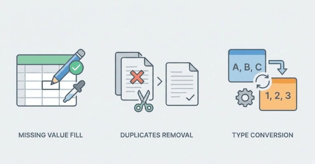
Q106. How do you identify and handle duplicate rows?
Pandas provides the duplicated method to identify duplicate rows, returning a boolean Series indicating which rows are duplicates. The drop_duplicates method removes duplicates, keeping the first occurrence by default. You can specify which columns to consider using the subset parameter, useful when only certain columns determine uniqueness. The keep parameter controls which duplicate to keep: first, last, or False to remove all duplicates. In machine learning, duplicates can bias models toward repeated examples, so identifying and handling them is crucial for data quality.
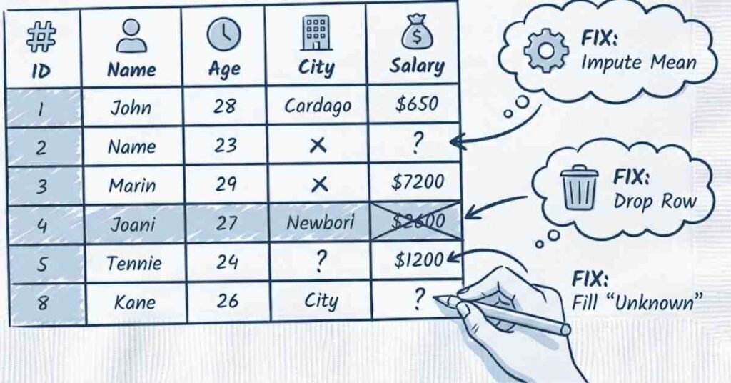
Q107. What are different strategies for handling missing data?
Several strategies exist for missing data. Deletion removes rows with missing values using dropna, simple but loses information. Mean or median imputation replaces missing values with column averages using fillna, preserving sample size but potentially distorting distributions. Forward fill carries the last valid value forward using fillna with method forward fill, useful for time series. Backward fill does the opposite. More sophisticated approaches use machine learning to predict missing values based on other features. The choice depends on how much data is missing, why it’s missing, and your model requirements.
Q108. How do you replace values in a DataFrame?
The replace method substitutes specified values with new ones. You can replace a single value across the entire DataFrame, or use a dictionary mapping old values to new ones. For specific columns, use bracket notation to select them first. The str.replace method handles string replacements within text columns, supporting regular expressions for pattern matching. In machine learning preprocessing, replace corrects data entry errors, standardizes category names, converts codes to meaningful values, or maps categorical values to numbers for modeling.
Q109. What is the difference between fillna and interpolate?
Both handle missing values but differently. fillna replaces missing values with specified constants, statistics like mean or median, or values from other rows using forward or backward fill. It’s simple and fast but doesn’t consider relationships between values. interpolate estimates missing values based on surrounding values using mathematical interpolation methods like linear, polynomial, or spline. It’s more sophisticated and works well for time series or ordered data where missing values should follow trends. Choose fillna for simple replacement and interpolate when missing values should reflect patterns in surrounding data.
Q110. How do you handle inconsistent data formats?
Inconsistent formats appear in many forms: dates in different formats, numbers with commas or currency symbols, inconsistent capitalization, or varying category names. The str accessor provides string methods for cleaning text columns like str.lower for consistent case, str.strip to remove whitespace, and str.replace for pattern replacement. The pd.to_datetime function converts various date formats to datetime objects, with the format parameter specifying the expected pattern. For numbers, str.replace removes unwanted characters before converting to numeric type. Systematic cleaning ensures your features are interpretable by machine learning algorithms.
4.4 Data Wrangling Strategies
Q111. What is the melt function and when do you use it?
The melt function transforms wide-format data into long format, also called unpivoting. Wide format has many columns representing different variables or time periods. Long format has fewer columns with one row per observation. You specify id_vars for columns to keep and value_vars for columns to melt. This creates a new DataFrame with identifiers, a variable column naming which original column the value came from, and a value column. Melting is useful when algorithms expect long format or when you need to plot or analyze data where current columns should be values of a variable.
Q112. How does the pivot function work?
Pivot does the opposite of melt, transforming long-format data into wide format. You specify which column’s values become the new index, which column’s values become new columns, and which column’s values fill the resulting table. This reshapes data from one row per observation to one row per entity with observations as columns. In machine learning, pivot creates feature matrices from transactional data, converts time series from long to wide format, or restructures datasets for specific algorithm requirements.
Q113. What is the groupby operation?
The groupby operation splits data into groups based on column values, applies a function to each group, and combines results. It follows the split-apply-combine pattern. After grouping with df.groupby, you call aggregation functions like sum, mean, or count. For example, grouping sales data by region then calculating average sales per region. You can group by multiple columns, creating hierarchical groups. In machine learning, groupby creates aggregate features, computes group-level statistics, analyzes model performance by segments, or prepares data for certain algorithms.
Q114. How do you merge and join DataFrames?
Merging combines DataFrames based on common columns or indices, similar to SQL joins. The merge function takes two DataFrames and specifies how to join them. Inner join keeps only rows with matches in both DataFrames. Left join keeps all rows from the left DataFrame. Right join keeps all from the right. Outer join keeps all rows from both. You specify which columns to join on using the on parameter. When column names differ, use left_on and right_on. In machine learning, merging combines features from different sources, adds target variables to feature data, or enriches datasets with external information.
Q115. What is the concat function used for?
Concat stacks DataFrames together vertically or horizontally. Vertical concatenation adds rows from one DataFrame below another, useful for combining datasets with the same columns. Horizontal concatenation adds columns side by side, useful for adding new features. The axis parameter controls direction: zero for vertical, one for horizontal. The ignore_index parameter resets the index in the result. Unlike merge, concat doesn’t require common columns; it simply stacks data. In machine learning, concat combines training batches, adds engineered features, or assembles final datasets from multiple preprocessing steps.
4.5 Data Selection and Filtering
Q116. What is the difference between loc and iloc?
Both select subsets of DataFrames but use different indexing. loc uses label-based indexing, selecting rows and columns by their names. You write df.loc bracket row_label comma column_label bracket. iloc uses position-based indexing, selecting by integer positions like NumPy arrays. You write df.iloc bracket row_position comma column_position bracket. loc is more intuitive when you know names, while iloc is useful for positional access. For slicing, loc includes both endpoints while iloc excludes the end. Understanding both is essential for flexible data selection in machine learning preprocessing.
Q117. How do you filter rows based on conditions?
You filter by creating boolean Series from conditions then using them to index DataFrames. Write conditions like df bracket quote age quote greater than 30, which returns a boolean Series. Use this inside brackets like df bracket df bracket quote age quote greater than 30 bracket to get filtered rows. Combine multiple conditions with ampersand for and, vertical bar for or, and tilde for not. Remember to parenthesize each condition. In machine learning, filtering selects training samples meeting criteria, removes outliers, creates subsets for analysis, or separates data by class.
Q118. What is the query method?
The query method filters rows using string expressions, providing cleaner syntax than boolean indexing. You write conditions as strings like df.query quote age greater than 30 and salary less than 100000 quote. This is more readable, especially with complex conditions. You can reference variables from your environment using the at symbol. The query method uses the same operators as Python but in string form. It’s particularly useful when conditions come from user input or configuration files, though boolean indexing is more common in production code.
Q119. How do you select rows by index position?
Use iloc with integer positions or slices. df.iloc bracket five bracket selects the sixth row. df.iloc bracket ten colon twenty bracket selects rows ten through nineteen. Negative indices count from the end. You can pass lists of positions like df.iloc bracket bracket zero comma five comma ten bracket bracket. For both rows and columns, separate with comma like df.iloc bracket zero colon ten comma zero colon five bracket for first ten rows and first five columns. Position-based selection is essential when row order matters or when you need to sample specific positions.
Q120. What are boolean masks and how do you use them?
Boolean masks are Series or arrays of True and False values that select rows where the value is True. Create masks from conditions, then use them to index DataFrames. You can combine masks using logical operators, save masks as variables for reuse, or create complex masks using multiple conditions. For example, create a mask for valid data, another for training set, then combine them to select valid training samples. Masks make complex selection logic clearer and enable reusing selection criteria across different operations.
Chapter 5: Data Visualization with Matplotlib
5.1 Basic Plotting Techniques
Q121. Why is data visualization important in machine learning?
Data visualization helps you understand your data before modeling, identify patterns and relationships, detect outliers and anomalies, and communicate results effectively. Visualizations reveal distributions, correlations, and trends that numbers alone don’t show. Before training models, plots help you decide on preprocessing steps and feature engineering. During training, visualizations track learning progress and diagnose problems. After training, plots communicate model behavior and predictions to stakeholders. Good visualization skills make you a more effective machine learning practitioner by enabling data-driven decisions.
Q122. How do you create a basic line plot with Matplotlib?
Start by importing Matplotlib with import matplotlib.pyplot as plt. Create a figure and axes with fig comma ax equals plt.subplots. Plot data with ax.plot passing x and y values. Add labels with ax.set_xlabel and ax.set_ylabel. Add a title with ax.set_title. Display the plot with plt.show. You can customize line color, style, and width using parameters. Multiple lines on one plot help compare different models or features. In machine learning, line plots visualize training curves, showing how loss decreases over epochs.
Q123. What are scatter plots and when do you use them?
Scatter plots display individual data points as dots in two-dimensional space, with x and y coordinates. Create them with ax.scatter passing x and y arrays. They reveal relationships between two variables, showing correlation, clustering, or patterns. In machine learning, scatter plots visualize feature relationships, show actual versus predicted values to assess model accuracy, display dimensionality reduction results like PCA, or identify outliers as points far from clusters. Color and size parameters add additional dimensions, encoding class labels or confidence scores.
Q124. How do you create bar charts and histograms?
Bar charts display categorical data with rectangular bars. Use ax.bar passing categories and heights. They compare quantities across categories like model accuracy for different algorithms. Histograms show distribution of continuous data by binning values and counting frequency. Use ax.hist passing data and number of bins. They reveal data distribution shape, helping you assess normality, identify skewness, or detect multiple modes. In machine learning, histograms visualize feature distributions, understand class imbalance, examine prediction distributions, or analyze residual distributions to validate model assumptions.
Q125. What is the purpose of the plot title and axis labels?
Titles and labels make plots self-explanatory. The title summarizes what the plot shows, the x-axis label identifies the horizontal variable with units, and the y-axis label does the same for the vertical variable. Good labels enable viewers to understand plots without additional explanation. In machine learning reports or presentations, clear labeling is professional and ensures your audience understands your visualizations. Include units where appropriate, use descriptive names instead of variable codes, and make titles informative about what insight the plot reveals.
5.2 Customizing Plots and Figures
Q126. How do you change colors and line styles?
Matplotlib offers extensive customization. The color parameter accepts color names like red, hex codes like hashtag FF5733, or RGB tuples. The linestyle parameter sets line patterns: solid is default, dashed creates dashed lines, dotted creates dots. The marker parameter adds shapes at data points: circle creates circles, square creates squares. The linewidth parameter controls thickness. Combining these creates visually distinct plots when showing multiple series. In machine learning, color coding by class or model type makes comparison plots clearer.
Q127. What is the figure and axes object model?
Matplotlib uses a hierarchical object model. The figure is the entire window or page holding plots. Axes are individual plot areas within the figure, not to be confused with x and y axes. A figure can contain multiple axes subplots. You create both with plt.subplots returning figure and axes objects. This explicit object-oriented approach gives precise control over plot elements. For machine learning, this matters when creating complex visualizations with multiple subplots comparing different aspects of model performance or data distributions.
Q128. How do you add legends to plots?
Legends identify what each line or marker represents. When plotting, add a label parameter with a descriptive name. Then call ax.legend to display the legend box. The loc parameter controls position: upper right, lower left, et cetera. You can place legends outside the plot area by adjusting bbox_to_anchor. Good legends use concise, descriptive labels, don’t overlap data, and appear in consistent locations across related plots. In machine learning visualizations, legends distinguish between training and validation curves, different models, or various feature distributions.
Q129. What are figure size and DPI, and why do they matter?
Figure size determines plot dimensions in inches, specified with the figsize parameter as width comma height tuple when creating figures. DPI controls resolution in dots per inch. Larger figures accommodate more detail but take more space. Higher DPI creates sharper images but larger file sizes. For presentations, use larger figures with moderate DPI. For publications, use higher DPI for print quality. For notebooks, balance between readability and memory usage. In machine learning, appropriate sizing ensures plots are readable in reports and presentations.
Q130. How do you save plots to files?
Use plt.savefig or fig.savefig with a filename including extension. Common formats include PNG for raster images, SVG for vector graphics that scale perfectly, and PDF for documents. The dpi parameter controls resolution, bbox_inches equals tight removes excess whitespace, and transparent equals True makes backgrounds transparent. Save plots before calling plt.show, as showing sometimes clears figures. In machine learning workflows, saving plots preserves results for documentation, enables including visualizations in reports, and creates figures for papers or presentations.
5.3 Multiple Subplots Creation
Q131. How do you create multiple subplots in one figure?
Use plt.subplots with nrows and ncols parameters specifying the grid layout. This returns a figure and an array of axes objects. For example, fig comma axes equals plt.subplots two comma two creates a two-by-two grid. Access individual subplots with array indexing like axes bracket zero comma one bracket. This organizes related plots together, making comparisons easier. In machine learning, subplots show training and validation curves side by side, compare feature distributions across classes, or display multiple evaluation metrics together.
Q132. What is the difference between subplots and subplot?
plt.subplots with an s creates all subplots at once, returning a figure and axes array. It’s the modern, recommended approach. plt.subplot without an s creates one subplot at a time using MATLAB-style notation, requiring calling it multiple times with subplot position codes. subplots is cleaner and more Pythonic, giving you explicit handles to all axes upfront. subplot is older but still works. For machine learning visualizations, use subplots for cleaner, more maintainable code.
Q133. How do you adjust spacing between subplots?
Use fig.tight_layout to automatically adjust spacing, preventing overlapping labels and titles. For manual control, use fig.subplots_adjust with parameters like hspace for vertical spacing and wspace for horizontal spacing. Values are fractions of subplot size. Proper spacing makes subplot collections readable, ensuring titles don’t overlap neighboring plots and axis labels remain visible. In machine learning dashboards showing multiple metrics, good spacing maintains clarity even with many subplots.
Q134. Can you create subplots with different sizes?
Yes, using GridSpec provides flexible subplot arrangements. Import with from matplotlib.gridspec import GridSpec. Create a grid specification with desired proportions, then create axes occupying specific grid sections. This enables layouts like one large plot on top with two smaller plots below, or side-by-side plots with different widths. In machine learning, asymmetric layouts highlight primary visualizations while showing supporting plots smaller, or give more space to complex visualizations like confusion matrices.
Q135. How do you share axes between subplots?
The sharex and sharey parameters in plt.subplots make subplots share axes. Shared x-axes maintain the same horizontal range and zoom together. Shared y-axes do likewise vertically. This is perfect for comparing plots where alignment matters, like showing training curves for different models on the same scale. Changes to one subplot’s axis limits automatically apply to shared subplots. In machine learning, sharing axes ensures fair visual comparison between models or datasets.
Chapter 6: Machine Learning Fundamentals
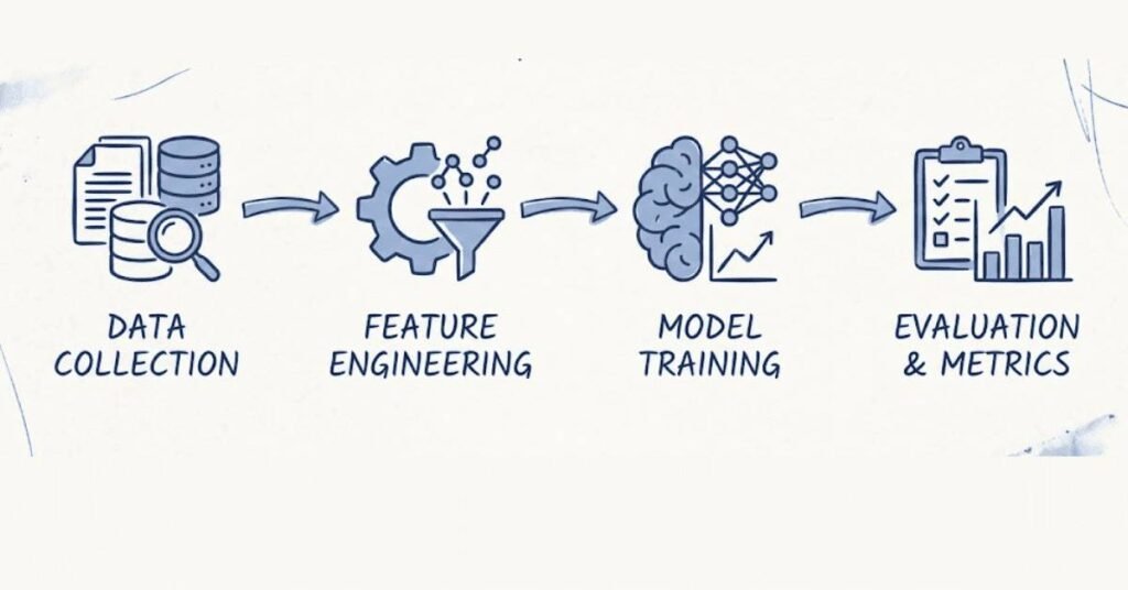
6.1 What is Machine Learning
Q136. Define machine learning in simple terms.
Machine learning is teaching computers to learn from experience without being explicitly programmed for every scenario. Instead of writing specific rules, you show the computer many examples, and it discovers patterns automatically. For instance, rather than programming every rule for recognizing cats in images, you show thousands of cat and non-cat images, and the algorithm learns distinguishing features. Machine learning powers recommendation systems, voice assistants, fraud detection, and countless applications where programming explicit rules would be impossible or impractical.
Q137. What are the main applications of machine learning?
Machine learning applications span virtually every industry. In healthcare, it diagnoses diseases and predicts patient outcomes. In finance, it detects fraud and automates trading. In retail, it recommends products and optimizes inventory. In transportation, it enables self-driving cars. In entertainment, it recommends movies and music. In manufacturing, it predicts equipment failures. In agriculture, it optimizes crop yields. The unifying theme is using data to make predictions, automate decisions, or discover insights that would be difficult or impossible manually.
Q138. How does machine learning differ from traditional programming?
Traditional programming involves writing explicit rules: if this condition then that action. You define all logic upfront. Machine learning flips this. You provide input-output examples, and the algorithm infers the rules automatically. Traditional programming works when rules are clear and don’t change. Machine learning excels when rules are too complex to code, like understanding natural language, or when rules change over time, like user preferences. The key shift is from programming rules to learning patterns from data.
Q139. What is the general workflow of a machine learning project?
A typical ML project follows these stages. First, define the problem and success criteria. Second, collect and explore data to understand what you’re working with. Third, prepare data through cleaning, transformation, and feature engineering. Fourth, choose and train models, experimenting with different algorithms. Fifth, evaluate models on held-out data to assess performance. Sixth, tune hyperparameters to optimize results. Seventh, validate with domain experts and additional testing. Finally, deploy the model to production and monitor its performance over time.
Q140. What skills are essential for machine learning practitioners?
Successful ML practitioners combine several skills. Programming proficiency, especially Python, is fundamental. Statistics and probability enable understanding algorithms and evaluation. Linear algebra and calculus underpin how algorithms work mathematically. Domain knowledge helps frame problems correctly and interpret results. Communication skills translate technical findings for non-technical stakeholders. Practical experience with data wrangling, visualization, and debugging is crucial since real projects involve messy data and unexpected issues. Continuous learning keeps skills current in this rapidly evolving field.
6.2 Types of Machine Learning Systems
Q141. What is supervised learning?
Supervised learning trains models using labeled data where each input has a corresponding output. You show the algorithm examples of correct answers, and it learns to map inputs to outputs. Classification predicts categorical labels like spam or not spam. Regression predicts continuous values like house prices. Common algorithms include linear regression, logistic regression, decision trees, and neural networks. Supervised learning is the most common type, used when you have historical data with known outcomes and want to predict outcomes for new data.
Q142. What is unsupervised learning?
Unsupervised learning works with unlabeled data where you don’t have predefined outputs. The algorithm discovers structure, patterns, or groupings automatically. Clustering groups similar items together, like segmenting customers by behavior. Dimensionality reduction finds simplified representations, like summarizing hundreds of features with a few components. Anomaly detection identifies unusual patterns. Unsupervised learning is valuable for exploration, finding hidden structure, preprocessing for supervised learning, or applications where labeling data is expensive or impossible.
Q143. What is reinforcement learning?
Reinforcement learning trains agents to make sequences of decisions by rewarding desired behaviors and penalizing undesired ones. The agent explores an environment, takes actions, receives rewards or penalties, and learns which actions maximize long-term reward. It’s similar to training a dog with treats and corrections. Applications include game playing like chess or Go, robotics where robots learn physical tasks, autonomous driving, and recommendation systems. Unlike supervised learning where correct answers are provided, reinforcement learning agents must discover successful strategies through trial and error.
Q144. What is semi-supervised learning?
Semi-supervised learning combines small amounts of labeled data with large amounts of unlabeled data. Labeling data is often expensive and time-consuming, but unlabeled data is abundant. The algorithm uses labeled data to learn initial patterns, then uses unlabeled data to refine and improve. This approach works when labeling every example is impractical but you can label some examples. Applications include text classification where reading and labeling millions of documents is infeasible, or medical imaging where expert labeling is expensive but vast unlabeled images exist.
Q145. What is transfer learning?
Transfer learning reuses knowledge from one task to help with a related task. Instead of training from scratch, you start with a model trained on a large dataset, then adapt it to your specific problem. For example, a model trained to recognize general objects can be fine-tuned to recognize specific medical conditions. This works because early layers learn general features like edges and textures that apply broadly. Transfer learning saves time and computational resources, works with smaller datasets, and often achieves better performance than training from scratch.
6.3 Supervised Learning Concepts
Q146. What is a training set?
The training set is the portion of data used to train your model, typically 60 to 80 percent of your total data. The algorithm sees these examples with their correct answers and adjusts its parameters to minimize prediction errors. The model learns patterns, relationships, and decision boundaries from this data. The quality and quantity of training data largely determines model performance. Too little data leads to poor learning. Biased or unrepresentative training data creates models that don’t generalize well to real-world situations.
Q147. What is a test set and why is it important?
The test set is held-out data that the model never sees during training, used to evaluate final performance. It simulates how the model will perform on new, unseen data in production. Test set performance is the ultimate measure of model quality because it reveals generalization ability. If training accuracy is high but test accuracy is low, the model overfit to training data. The test set should be representative of data the model will encounter in real use, matching the distribution and characteristics.
Q148. What is a validation set?
The validation set is a separate portion of data used during model development to tune hyperparameters and make model selection decisions. While the test set remains untouched until final evaluation, you use the validation set repeatedly during development. This prevents overfitting to the test set through repeated evaluation. Typical splits are 60 percent training, 20 percent validation, and 20 percent test. The validation set helps you choose between models, adjust learning rates, decide when to stop training, and make other decisions without contaminating the test set.
Q149. What is cross-validation?
Cross-validation evaluates models more robustly by training and testing multiple times on different data splits. The most common type is k-fold cross-validation where you divide data into k equal parts. You train k times, each time using k minus one parts for training and one part for validation, rotating which part is held out. Average the k validation scores for the final performance estimate. This gives more reliable performance estimates than a single split, especially with limited data, and reduces dependence on one particular train-test split.
Q150. What is stratification in train-test splitting?
Stratification ensures that class proportions remain consistent across training, validation, and test sets. Without stratification, random splitting might create imbalanced splits where some classes are over or underrepresented in different sets. For example, with 90 percent positive and 10 percent negative examples, random splitting might put most negatives in the training set, leaving few for testing. Stratified splitting maintains the 90-10 ratio in all sets. This prevents biased evaluation and ensures the model trains on representative data.
6.4 Unsupervised Learning Techniques
Q151. What is clustering and what are its applications?
Clustering groups similar data points together without predefined labels. Points in the same cluster are more similar to each other than to points in other clusters. Applications include customer segmentation where you group customers by purchasing behavior, image segmentation dividing images into regions, document organization grouping similar articles, anomaly detection where outliers don’t fit any cluster, and data exploration discovering natural groupings. Clustering helps you understand data structure, reduce complexity by working with groups instead of individuals, and find patterns you didn’t know existed.
Q152. What is dimensionality reduction?
Dimensionality reduction transforms high-dimensional data into lower dimensions while preserving important information. With hundreds or thousands of features, visualization is impossible and computation is slow. Reduction techniques find lower-dimensional representations that capture most variance or information. This enables visualization in two or three dimensions, speeds up algorithms, reduces storage requirements, and sometimes improves model performance by removing noise. It’s essential for working with high-dimensional data like images, text, or genomic data.
Q153. What is anomaly detection?
Anomaly detection identifies unusual patterns that deviate from normal behavior. It learns what normal looks like from data, then flags examples that don’t fit. Applications include fraud detection where unusual transactions are flagged, network intrusion detection identifying suspicious activity, equipment monitoring detecting impending failures, and quality control finding defective products. Anomalies are rare, making them hard to detect with standard classification since you rarely have enough anomaly examples for training. Unsupervised methods learn normal patterns, then flag deviations.
Q154. What are association rules?
Association rules discover relationships between variables in large datasets, particularly in retail transaction data. The classic example is market basket analysis finding which products are frequently bought together. Rules take the form if customers buy X then they also buy Y. Metrics like support measure how often itemsets appear, confidence measures how often the rule is true, and lift measures how much more likely items appear together than independently. Applications include product recommendation, store layout optimization, and understanding customer behavior patterns.
Q155. How does unsupervised learning help with supervised learning?
Unsupervised learning often preprocesses data for supervised learning. Dimensionality reduction creates better features by removing noise and redundancy. Clustering can generate features indicating which cluster each point belongs to, adding useful information. Anomaly detection identifies and removes outliers that might hurt supervised model training. Unsupervised pretraining in deep learning initializes network weights before supervised fine-tuning. Understanding data structure through unsupervised exploration helps you make better decisions about feature engineering and model selection.
Chapter 7: Classification Models
7.1 Binary Classification Fundamentals
Q156. What is binary classification?
Binary classification predicts one of two possible outcomes, like yes or no, true or false, positive or negative. Examples include spam detection where emails are spam or not spam, disease diagnosis where patients have the disease or don’t, and customer churn where customers leave or stay. Despite having only two classes, binary classification is fundamental to machine learning and covers countless real-world applications. Most classification algorithms work primarily as binary classifiers and extend to multiple classes through various strategies.
Q157. How do classification algorithms work conceptually?
Classification algorithms learn decision boundaries that separate different classes in feature space. During training, the algorithm examines labeled examples and finds patterns distinguishing classes. It might learn that spam emails contain certain words, occur at certain times, or have particular characteristics. The algorithm creates a mathematical function mapping input features to class probabilities or predictions. At prediction time, new examples are evaluated by this function, which determines which side of the decision boundary they fall on, assigning them to the appropriate class.
Q158. What is a decision boundary?
A decision boundary is the line, surface, or more complex shape that separates different classes in feature space. Points on one side are predicted as one class, points on the other side as another class. For linear models, the boundary is a straight line in two dimensions or a flat plane in higher dimensions. For non-linear models like neural networks or decision trees, boundaries can be curved or irregular. Visualizing decision boundaries helps you understand what your model learned and identify where it might make mistakes.
Q159. What is the difference between hard and soft classification?
Hard classification makes definitive predictions, assigning each example to exactly one class. The output is simply the predicted class label. Soft classification provides probability estimates for each class. Instead of just predicting spam or not spam, it might say 85 percent probability of spam. Soft predictions are more informative, allowing you to set custom decision thresholds, quantify confidence, and handle uncertain cases differently. Most algorithms support both by computing probabilities then choosing the highest as the hard prediction.
Q160. How do you choose between binary classification and regression?
The choice depends on your output variable. If it’s categorical with distinct classes like disease or no disease, use classification. If it’s continuous like predicting blood pressure values, use regression. Sometimes the distinction blurs. You could frame disease severity as multiple classes or as a continuous scale. Generally, use classification for inherently categorical outcomes where intermediate values don’t make sense, and regression for continuous outcomes where the exact value matters. Some problems can be approached either way depending on business requirements.
7.2 Performance Measurement Metrics
Q161. What is accuracy and when is it misleading?
Accuracy is the fraction of predictions that are correct, calculated as correct predictions divided by total predictions. It’s intuitive and commonly used but misleading with imbalanced classes. If 95 percent of emails aren’t spam, predicting everything as not spam achieves 95 percent accuracy while being completely useless for detecting spam. Accuracy treats all errors equally, which might not match business costs where false positives and false negatives have different consequences. For imbalanced problems or when error types have different costs, other metrics are more informative.
Q162. What is precision?
Precision measures what fraction of positive predictions are actually positive. It answers how many items labeled positive by your model are truly positive. Calculated as true positives divided by true positives plus false positives, it ranges from zero to one. High precision means few false alarms. Precision is critical when false positives are costly or annoying, like spam filtering where marking legitimate emails as spam frustrates users. Optimizing for precision reduces false positives but might increase false negatives.
Q163. What is recall?
Recall measures what fraction of actual positives your model finds. It answers how many truly positive items your model successfully identifies. Calculated as true positives divided by true positives plus false negatives, it ranges from zero to one. High recall means few missed positives. Recall is critical when false negatives are dangerous or costly, like disease screening where missing sick patients has serious consequences. Optimizing for recall reduces false negatives but might increase false positives.
Q164. How do precision and recall trade off?
Precision and recall often trade off inversely. Making your model more conservative in predicting positive increases precision because you only predict positive when very confident, but decreases recall because you miss positive cases where you’re less certain. Making your model more aggressive increases recall by catching more positives but decreases precision through more false alarms. The trade-off is controlled by the decision threshold for classification. The optimal balance depends on the relative costs of false positives versus false negatives.
Q165. What is the F1 score?
The F1 score combines precision and recall into a single metric using their harmonic mean. It’s calculated as two times precision times recall divided by precision plus recall. The F1 score ranges from zero to one, where one is perfect precision and recall. It’s useful when you need a single number balancing both metrics, especially with imbalanced classes where accuracy is misleading. The F1 score penalizes extreme values, so you need both reasonable precision and recall to score well. For different cost structures, you can use weighted variants like F-beta scores.
7.3 Accuracy and Its Limitations
Q166. Why is accuracy problematic for imbalanced datasets?
With imbalanced datasets where one class vastly outnumbers others, accuracy provides false confidence. A model predicting only the majority class achieves high accuracy while being useless for the minority class. If 99 percent of transactions aren’t fraudulent, predicting everything as legitimate achieves 99 percent accuracy but catches zero fraud. The problem is accuracy weights all examples equally, so the majority class dominates the metric. For imbalanced problems, use metrics like precision, recall, F1, or area under ROC curve that provide meaningful insight into minority class performance.
Q167. When is accuracy an appropriate metric?
Accuracy works well when classes are balanced, all prediction errors have similar costs, and you care equally about performance on all classes. For example, classifying images of different animals where each animal appears equally often and all misclassifications are equally problematic. Accuracy is also appropriate as one metric among several, giving an overall sense of correctness. However, even with balanced classes, if false positives and false negatives have different costs, other metrics provide better guidance for model development.
Q168. How do you interpret accuracy in context?
Always compare accuracy to baseline performance. Random guessing achieves 50 percent accuracy for balanced binary problems. Always predicting the majority class achieves accuracy equal to the majority class fraction. Your model should substantially exceed these baselines. Consider domain requirements: medical diagnosis might need 99 percent accuracy, while movie recommendations work fine with 70 percent. Report accuracy alongside other metrics that reveal performance nuances. Context about class balance, error costs, and business requirements determines whether a given accuracy level is acceptable.
Q169. What are balanced accuracy and other alternatives?
Balanced accuracy averages recall across classes, giving equal weight to each class regardless of size. This makes it suitable for imbalanced problems. It’s calculated as the average of true positive rate and true negative rate. Cohen’s kappa measures agreement beyond chance, useful when classes are imbalanced. Matthews correlation coefficient considers all confusion matrix elements and is regarded as balanced even with imbalanced data. These alternatives provide more reliable performance assessment than accuracy for imbalanced problems.
Q170. How does class imbalance affect model training?
Class imbalance causes models to bias toward the majority class because predicting the majority class minimizes training loss. The model doesn’t learn minority class patterns well since they contribute little to overall error. Solutions include resampling where you oversample the minority class or undersample the majority class, using class weights that penalize minority class errors more heavily, choosing appropriate evaluation metrics that focus on minority class performance, or using specialized algorithms designed for imbalanced data. Addressing imbalance is crucial for good minority class performance.
7.4 Confusion Matrix Interpretation
Q171. What is a confusion matrix?
A confusion matrix is a table showing predicted versus actual classes, revealing exactly where your model makes mistakes. For binary classification, it’s a two-by-two table with true positives, false positives, true negatives, and false negatives. Each cell counts how many examples fell into that category. True positives are correctly predicted positives, false positives are negatives wrongly predicted as positive, true negatives are correctly predicted negatives, and false negatives are positives wrongly predicted as negative. This complete picture helps you understand model behavior beyond simple accuracy.
Q172. How do you calculate metrics from a confusion matrix?
All classification metrics derive from confusion matrix values. Accuracy equals true positives plus true negatives divided by all examples. Precision equals true positives divided by true positives plus false positives. Recall equals true positives divided by true positives plus false negatives. Specificity equals true negatives divided by true negatives plus false positives. False positive rate equals false positives divided by false positives plus true negatives. Having the confusion matrix lets you compute any metric and understand exactly where errors occur.
Q173. How do you interpret patterns in confusion matrices?
Confusion matrix patterns reveal systematic errors. High false positives with low false negatives means your model is too aggressive, predicting positive too often. The opposite pattern means it’s too conservative. If one specific class is frequently confused with another, those classes might be genuinely similar, suggesting you need better features to distinguish them. Diagonal dominance shows good performance, while off-diagonal concentration indicates problems. Examining which examples fall in which cells guides improvement efforts.
Q174. How do confusion matrices extend to multiclass problems?
For multiclass problems, the confusion matrix becomes larger with one row and column per class. Rows represent actual classes, columns represent predicted classes. The diagonal shows correct predictions for each class. Off-diagonal cells show confusions between specific class pairs. You can calculate per-class precision and recall, revealing which classes perform well and which are problematic. Large off-diagonal values between specific classes indicate those classes are hard to distinguish. The confusion matrix visualizes performance across all classes simultaneously.
Q175. What visualization techniques help interpret confusion matrices?
Heatmaps color-code confusion matrix cells by count or proportion, making patterns visually apparent. Darker colors might represent more examples, highlighting where most errors occur. Normalization by row shows what percentage of each actual class gets predicted as each class, useful for understanding per-class recall. Normalization by column shows what percentage of predictions for each class are correct, useful for precision. Sorting classes by similarity can reveal structure. These visualizations make confusion matrices more interpretable, especially for many classes.
Chapter 8: Regression Models
8.1 Linear Regression Basics
Q176. What is linear regression?
Linear regression models the relationship between input features and a continuous output as a straight line or hyperplane. It assumes the output is a weighted sum of inputs plus a constant, written as y equals weight one times x one plus weight two times x two and so on plus bias. The algorithm learns optimal weights by minimizing the difference between predictions and actual values. Despite its simplicity, linear regression is widely used, interpretable, fast to train, and effective for many problems. It serves as the foundation for understanding more complex models.
Q177. What are the assumptions of linear regression?
Linear regression assumes several things about data. Linearity means the relationship between features and target is linear. Independence means observations don’t affect each other. Homoscedasticity means error variance is constant across all feature values. Normality means errors are normally distributed. No multicollinearity means features aren’t highly correlated with each other. Violations of these assumptions can degrade performance or make interpretations incorrect. Checking assumptions helps you understand when linear regression is appropriate and when to try other approaches.
Q178. How do you interpret coefficients in linear regression?
Each coefficient represents the change in predicted output for a one-unit increase in that feature, holding other features constant. Positive coefficients mean the feature increases the prediction, negative coefficients mean it decreases the prediction. Larger absolute values indicate stronger effects. The bias term is the predicted value when all features are zero. Interpretation becomes more complex with feature scaling or engineering. Standardizing features makes coefficients comparable in importance. Linear regression’s interpretability is a major advantage, helping you understand what drives predictions.
Q179. What is the difference between simple and multiple linear regression?
Simple linear regression has one input feature, modeling the output as a straight line in two-dimensional space. Multiple linear regression has multiple input features, modeling the output as a hyperplane in higher-dimensional space. The mathematics and principles are identical; only the dimensionality differs. Multiple regression is more common in machine learning since most problems have many features. It can capture how different features jointly affect the output and account for correlations between features.
Q180. What is polynomial regression?
Polynomial regression extends linear regression by including polynomial terms like x squared or x cubed as features. This allows modeling curved relationships while using the same linear regression algorithm. You create polynomial features from original features, then apply linear regression to the expanded feature set. The model is still linear in its parameters but can fit non-linear patterns in data. However, high-degree polynomials can overfit. Polynomial regression is useful when relationships are curved but not extremely complex.
8.2 Gradient Descent Algorithm
Q181. What is gradient descent?
Gradient descent is an optimization algorithm that finds model parameters minimizing the loss function. It starts with random parameters, calculates how the loss changes with each parameter using derivatives, then adjusts parameters in the direction that decreases loss. This process repeats iteratively until the loss stops improving significantly. The name comes from descending down the gradient or slope toward the minimum. Gradient descent is fundamental to training most machine learning models, especially neural networks where analytical solutions don’t exist.
Q182. What is a loss function?
A loss function measures how wrong your model’s predictions are, assigning a numeric penalty to errors. For regression, mean squared error calculates the average squared difference between predictions and actual values. For classification, cross-entropy measures how different predicted probabilities are from actual classes. The loss function translates the abstract goal of accurate predictions into a concrete number that optimization algorithms can minimize. Choosing the right loss function depends on your problem type and what kind of errors you want to penalize.
Q183. What is the learning rate?
The learning rate controls how big a step gradient descent takes when updating parameters. Large learning rates make big jumps, potentially converging faster but risking overshooting the minimum and oscillating. Small learning rates make tiny steps, converging reliably but very slowly. Choosing an appropriate learning rate is crucial for efficient training. Too large causes instability, too small wastes time. Typical values range from 0.001 to 0.1. Techniques like learning rate schedules decrease the rate during training, taking large steps initially then fine-tuning with small steps.
Q184. What are local minima and global minima?
The global minimum is the point where the loss function has its absolute lowest value. Local minima are points where the loss is lower than nearby points but not the absolute lowest. In a hilly landscape, the global minimum is the deepest valley while local minima are smaller dips. Gradient descent can get stuck in local minima, finding decent but not optimal solutions. For convex functions like linear regression loss, all local minima are global. For non-convex functions like neural network loss, many local minima exist, though in practice they’re often acceptable solutions.
Q185. How do you know when to stop gradient descent?
Several stopping criteria exist. You can set a maximum number of iterations and stop when reached. You can monitor loss and stop when it changes by less than some threshold between iterations, indicating convergence. You can stop when the gradient magnitude becomes very small, meaning you’re at a flat point. You can use early stopping where you monitor validation loss and stop when it stops improving, preventing overfitting. Combining criteria provides robust stopping behavior. The goal is stopping when further training doesn’t meaningfully improve the model.
8.3 Batch Gradient Descent
Q186. What is batch gradient descent?
Batch gradient descent computes the gradient using the entire training set for each update. It calculates the loss on all examples, computes gradients by averaging over all examples, then updates parameters once. This provides an accurate gradient estimate pointing toward the true minimum. Batch gradient descent converges smoothly but can be slow with large datasets since each iteration requires processing all data. It also requires loading the entire dataset into memory. Despite these limitations, it’s conceptually the cleanest version of gradient descent and works well for small to medium datasets.
Q187. What are the advantages of batch gradient descent?
Batch gradient descent has several advantages. The gradient estimates are accurate since they use all data, leading to stable convergence directly toward the minimum. Updates are large and meaningful since they reflect all examples. For convex problems, convergence to the global minimum is guaranteed. The algorithm is deterministic, producing the same results each run. It’s easy to understand and implement. For small datasets where memory isn’t a concern, batch gradient descent is often the best choice.
Q188. What are the disadvantages of batch gradient descent?
The main disadvantage is computational cost. With millions of examples, computing gradients over all data for every update is prohibitively expensive. Memory requirements can exceed available RAM. Convergence is slow on large datasets since you make only one update per full dataset pass. Updates become increasingly expensive as data grows. For these reasons, batch gradient descent is rarely used with big data despite its theoretical appeal. Modern deep learning almost exclusively uses variants that process data in smaller batches.
Q189. How does batch size affect training?
Batch size trades off between computational efficiency and gradient accuracy. Larger batches provide more accurate gradient estimates, leading to stabler updates and potentially better convergence. They also utilize hardware efficiently. However, they require more memory and provide fewer updates per epoch. Smaller batches make more frequent updates, allowing faster learning and sometimes better generalization. They also add noise that can help escape local minima. The optimal batch size depends on dataset size, model complexity, and hardware capabilities, often found experimentally.
Q190. What hardware considerations affect batch gradient descent?
Modern hardware significantly impacts training efficiency. GPUs excel at parallel computation, processing entire batches simultaneously much faster than CPUs. This makes batch processing efficient. However, GPU memory limits maximum batch size. TPUs designed specifically for machine learning offer even more parallelism. CPUs handle small batches but struggle with large ones. Multi-core CPUs parallelize across batches. The interaction between algorithm and hardware determines actual training speed. Optimizing batch size and implementation for your specific hardware maximizes efficiency.
8.4 Stochastic Gradient Descent
Q191. What is stochastic gradient descent?
Stochastic gradient descent or SGD updates parameters after each individual example rather than after the entire dataset. For each example, it computes the gradient of loss for just that example and updates parameters immediately. This makes updates very frequent and fast. The word stochastic means random, referring to the random order in which examples are processed. SGD trades gradient accuracy for speed, making much more progress per unit time than batch gradient descent. It’s become the standard for large datasets and deep learning.
Q192. Why is SGD faster than batch gradient descent?
SGD is faster because each update requires processing only one example instead of thousands or millions. You make an update instantly, move to the next example, update again, and so on. With a million examples, batch gradient descent makes one update while SGD makes a million updates. Even though each SGD update is less accurate, the sheer number of updates overwhelms this disadvantage. The model improves much faster in wall-clock time. For large datasets, SGD can converge before batch gradient descent completes even one iteration over the data.
Q193. What is the disadvantage of SGD?
SGD’s gradient estimates are noisy since they’re based on single examples that might not represent the overall data distribution. Updates jump around rather than smoothly descending toward the minimum. Training curves show high variance with loss bouncing up and down while generally decreasing. This noise can prevent converging exactly to the minimum, leaving the model oscillating nearby. The randomness makes training non-deterministic, producing slightly different results each run. The learning rate often needs careful tuning to balance speed and stability.
Q194. How does SGD help escape local minima?
The noise in SGD’s gradient estimates can be beneficial. If the model gets stuck in a shallow local minimum, noisy updates can bounce it out, potentially finding better minima. This stochastic exploration is especially valuable for non-convex problems like neural networks with many local minima. The randomness prevents getting trapped and encourages finding broader, flatter minima that generalize better. However, too much noise prevents converging at all. The balance between exploration and exploitation determines training success.
Q195. Should you shuffle data in SGD?
Yes, you should shuffle data before each epoch in SGD. Without shuffling, if your data has patterns in its order like all examples of one class together, SGD updates would be biased. The model would see batches of similar examples, leading to oscillating updates as it overfits to each class then the next. Shuffling ensures examples are processed in random order, making gradients more representative and training more stable. This is standard practice and significantly improves convergence.
8.5 Mini-Batch Gradient Descent
Q196. What is mini-batch gradient descent?
Mini-batch gradient descent combines advantages of batch and stochastic gradient descent by updating parameters after processing a small batch of examples instead of one or all. Typical batch sizes range from 32 to 512 examples. You compute the gradient averaged over the mini-batch, then update parameters. This provides more accurate gradients than SGD while being much faster than batch gradient descent. Mini-batch is now the standard approach in deep learning, offering the best trade-off between convergence stability and computational efficiency.
Q197. How do you choose batch size?
Batch size is a hyperparameter requiring tuning. Powers of two like 32, 64, 128, or 256 are common because they align well with computer memory architecture. Larger batches utilize GPU parallelism better but require more memory. Smaller batches make more frequent updates and sometimes generalize better. Very large batches may converge to sharper minima that generalize poorly. Dataset size matters: use smaller batches for small datasets, larger for big data. Start with common values like 32 or 64, then experiment based on memory constraints and convergence behavior.
Q198. What is an epoch?
An epoch is one complete pass through the entire training dataset. If you have 10,000 examples and a batch size of 100, one epoch involves 100 mini-batch updates. Training typically runs for multiple epochs, repeatedly cycling through the data. Models learn progressively with each epoch, extracting more subtle patterns. Early epochs make rapid progress, later epochs fine-tune. The number of epochs is another hyperparameter, determined by monitoring validation performance. Too few epochs means underfitting, too many means overfitting.
Q199. How do mini-batches enable parallelization?
Modern hardware processes multiple examples simultaneously. GPUs have thousands of cores handling different computations in parallel. Processing a mini-batch involves the same operations on different examples, perfect for parallelization. Forward propagation, gradient computation, and other operations run simultaneously on all examples in a batch. This means processing 64 examples in a batch takes barely longer than processing one example, dramatically speeding up training. Optimizing batch size to hardware capabilities maximizes throughput.
Q200. What is the difference between batch size and number of iterations?
Batch size is how many examples you process before updating parameters. Number of iterations is how many updates you make. For a dataset with 10,000 examples and batch size 100, one epoch involves 100 iterations. These concepts are related but distinct. You choose batch size based on memory and hardware capabilities. Number of iterations depends on dataset size and batch size. Understanding this relationship helps you estimate training time and properly configure your training loops.
8.6 Polynomial Regression
Q201. When should you use polynomial regression?
Use polynomial regression when the relationship between features and target is curved rather than straight. If scatter plots show curved patterns, polynomial features can capture these relationships. However, be cautious with high-degree polynomials as they can overfit dramatically, creating wild curves that fit training data perfectly but fail on new data. Typically, degree two or three polynomials work well. Beyond that, you’re usually better off with more sophisticated models like decision trees or neural networks that handle non-linearity naturally.
Q202. How do you create polynomial features?
Create polynomial features by raising original features to different powers and creating interaction terms. For features x1 and x2, a degree-two polynomial includes x1, x2, x1 squared, x2 squared, and x1 times x2. Scikit-learn provides PolynomialFeatures that automatically generates these. You specify the degree, and it creates all combinations up to that degree. Then you use these expanded features with regular linear regression. The model becomes non-linear in the input space while remaining linear in its parameters, allowing efficient optimization.
Q203. What are interaction terms?
Interaction terms are products of different features, capturing how features jointly affect the output. For example, in house pricing, size times location might be important because a large house matters more in good locations. The interaction term size multiplied by location rating captures this joint effect that neither feature alone represents. Polynomial regression automatically creates interaction terms. You can also manually create specific interactions based on domain knowledge. Interactions often improve model performance when combined effects exist.
Q204. What problems can high-degree polynomials cause?
High-degree polynomials create extremely complex curves that overfit training data. They fit every bump and wiggle in your training examples, including noise, then fail miserably on new data. Predictions can shoot to extreme values outside your training data range. The model becomes unstable with small changes in data causing large changes in predictions. Computation becomes expensive as the number of features explodes exponentially with degree. Generally, keep polynomial degrees low or use regularization to control complexity.
Q205. How does regularization help with polynomial regression?
Regularization penalizes large coefficients, preventing the wild oscillations that high-degree polynomials can produce. Even with many polynomial terms, regularization keeps most coefficients small, effectively selecting which terms matter. Ridge or Lasso regularization combined with polynomial features often works better than restricting polynomial degree. This approach lets you include many potential features while automatically controlling complexity. The regularization parameter controls the trade-off between fitting training data and keeping the model smooth.
8.7 Regularized Linear Models
Q206. What is regularization and why is it needed?
Regularization adds a penalty to the loss function based on model complexity, typically the magnitude of coefficients. This discourages overly complex models that fit training data perfectly but generalize poorly. Without regularization, models with many features can become unstable, with huge coefficients that amplify small input changes into large prediction changes. Regularization enforces simplicity, leading to models that work better on new data. It’s especially important when you have many features relative to training examples or when features are correlated.
Q207. What is Ridge regression?
Ridge regression adds a penalty proportional to the sum of squared coefficients to the loss function. This L2 regularization shrinks all coefficients toward zero but never exactly to zero. The regularization strength is controlled by a parameter alpha where larger values create stronger regularization and smaller coefficients. Ridge works well when many features contribute small amounts to predictions. It handles multicollinearity by distributing weight among correlated features rather than putting all weight on one. Ridge has a closed-form solution, making it computationally efficient.
Q208. What is Lasso regression?
Lasso regression uses L1 regularization, adding a penalty proportional to the absolute value of coefficients. Unlike Ridge, Lasso can shrink coefficients exactly to zero, effectively performing feature selection by eliminating unimportant features. This creates sparse models with few non-zero coefficients, which are interpretable and efficient. Lasso is powerful when you suspect only a few features truly matter. However, it can be unstable with correlated features, arbitrarily selecting one and zeroing others. Lasso requires iterative optimization without a closed-form solution.
Q209. How do you choose between Ridge and Lasso?
Choose Lasso when you want feature selection and believe many features are irrelevant. The resulting sparse model is interpretable and efficient. Choose Ridge when you believe most features contribute and want to keep them all but control their magnitudes. Ridge is more stable with correlated features. Elastic Net combines both penalties, offering a middle ground that performs feature selection while handling correlated features better than Lasso alone. Try all three and use cross-validation to select the best for your specific data.
Q210. What is the regularization parameter and how do you tune it?
The regularization parameter, often called alpha or lambda, controls regularization strength. Zero means no regularization, producing standard linear regression. Large values create strong regularization with small coefficients, potentially underfitting. You tune this hyperparameter using cross-validation, trying different values and selecting the one with best validation performance. Common practice is trying logarithmically spaced values like 0.001, 0.01, 0.1, 1, 10, 100. Scikit-learn provides RidgeCV and LassoCV that automate this tuning process.
8.8 Ridge Regression Implementation
Q211. How do Ridge regression coefficients behave as alpha increases?
As alpha increases, all coefficients shrink toward zero smoothly but never reach exactly zero. Large coefficients shrink faster than small ones, so their magnitudes become more similar. Features with less predictive power shrink more. Eventually with very large alpha, all coefficients become negligible and predictions approach the mean of the training data. Plotting coefficient paths showing how each coefficient changes with alpha reveals which features the model considers most important, as they resist shrinking longer.
Q212. Does Ridge regression require feature scaling?
Yes, Ridge regression is sensitive to feature scale. The penalty is based on coefficient magnitude, and coefficients depend on feature scale. Features with larger scales naturally get smaller coefficients, so they’re penalized less. This means Ridge would effectively apply different regularization strengths to different features based on their scales, which is unintended. Always standardize features before Ridge regression so all features have equal importance in the penalty term. This ensures fair regularization across all features.
Q213. How does Ridge regression handle multicollinearity?
Ridge regression handles multicollinearity well by distributing weight among correlated features rather than making the optimization unstable. When features are correlated, standard linear regression can produce huge coefficients with opposite signs that nearly cancel out. Ridge penalizes these large coefficients, stabilizing the solution. It finds coefficients that achieve good predictions while keeping magnitudes reasonable. The model becomes less sensitive to small data changes, making predictions more reliable. This is a major advantage of Ridge over ordinary linear regression.
Q214. Can Ridge regression be used for classification?
Ridge regression is primarily for regression problems predicting continuous values. However, Ridge regularization can be applied to logistic regression for classification, creating Ridge Logistic Regression. The same L2 penalty is added to the logistic loss function, providing similar benefits of controlling coefficient magnitudes and handling multicollinearity. Scikit-learn’s LogisticRegression includes Ridge regularization by default. The principles are the same, just applied to a different base model.
Q215. What is the computational complexity of Ridge regression?
Ridge regression with the closed-form solution has similar complexity to ordinary linear regression, roughly cubic in the number of features. For large datasets, iterative solvers can be more efficient. The advantage is that Ridge converges in one step with the analytical solution. For very large problems, specialized algorithms like coordinate descent provide efficiency. Overall, Ridge is computationally practical for most problems, and the small overhead compared to ordinary regression is usually worthwhile for improved generalization.
8.9 Lasso Regression Techniques
Q216. How does Lasso achieve feature selection?
Lasso’s L1 penalty creates sparse solutions where many coefficients equal exactly zero. The absolute value function has a corner at zero, and during optimization, coefficients tend to hit this corner and stay there. Geometrically, the L1 constraint region has corners aligned with axes, so the optimal solution often lands on these corners where some coordinates are zero. Features with coefficients zeroed out are effectively removed from the model. This automatic feature selection is Lasso’s signature advantage.
Q217. What happens when features are correlated in Lasso?
Lasso can behave unstably with highly correlated features. It tends to arbitrarily select one feature from a correlated group and zero out others, even when all contain similar information. Which feature gets selected can change with small data variations. This makes interpretation difficult and can hurt performance if the selected feature happens to have more noise. Elastic Net addresses this by blending L1 and L2 penalties, encouraging grouped selection of correlated features while maintaining some sparsity.
Q218. How do you interpret Lasso coefficients?
Non-zero Lasso coefficients indicate features the model selected as important. Their magnitudes and signs show the strength and direction of effects, similar to ordinary regression. Zero coefficients mean those features were deemed unimportant given the regularization strength. However, interpretation requires caution because feature selection depends on alpha, and correlated features may be arbitrarily included or excluded. Consider the stability of selections across different alpha values or data subsets before drawing strong conclusions about feature importance.
Q219. What is the coordinate descent algorithm for Lasso?
Coordinate descent optimizes one coefficient at a time while holding others fixed, cycling through all coefficients repeatedly. For Lasso, this is efficient because updating a single coefficient with L1 regularization has a simple closed-form solution involving soft thresholding. The algorithm iterates through coefficients, updating each to its optimal value given current values of others, and repeats until convergence. This approach is much faster than general-purpose optimizers for Lasso and is the standard method used in implementations like scikit-learn.
Q220. Can Lasso regression handle more features than samples?
Lasso can work with high-dimensional data where features outnumber samples, unlike ordinary regression which becomes unstable or impossible. The regularization prevents overfitting even with many features, and feature selection reduces the effective model complexity. However, Lasso selects at most as many features as samples, so with far more features than samples, many potentially useful features must be zeroed out. For extreme high-dimensional problems, specialized methods or more aggressive regularization may be needed.
8.10 Early Stopping Strategies
Q221. What is early stopping?
Early stopping halts training before convergence to prevent overfitting. You monitor validation performance during training and stop when it stops improving or starts degrading. This works because models typically fit training data progressively, learning general patterns first then overfitting to noise later. By stopping at the point of best validation performance, you get a model that generalizes well. Early stopping is simple, effective, and commonly used with iterative algorithms like gradient descent and neural network training.
Q222. How do you implement early stopping?
Track validation loss or accuracy during training. After each epoch or several iterations, evaluate on validation data and record performance. If validation performance doesn’t improve for a specified number of consecutive epochs called patience, stop training and restore the model to the point of best validation performance. For example, with patience of 10, if validation loss doesn’t decrease for 10 consecutive epochs, training stops and the model from the best epoch is kept. This prevents training from continuing into overfitting territory.
Q223. What patience value should you use?
Patience is a hyperparameter requiring tuning. Too small and you stop prematurely before reaching good solutions. Too large and you might overfit before stopping. Typical values range from 5 to 50 epochs depending on dataset size and model complexity. Larger datasets and simpler models might use smaller patience. Complex models on small data might need larger patience to ensure convergence. Start with medium values like 10 to 20 and adjust based on training curves showing when overfitting typically begins.
Q224. Is early stopping a form of regularization?
Yes, early stopping acts as regularization by limiting model complexity implicitly. Instead of directly penalizing parameter magnitudes like Ridge or Lasso, it limits optimization iterations. The effect is similar because the model doesn’t reach the point of fitting noise perfectly. Early stopping is sometimes called implicit regularization. It can be combined with explicit regularization like weight penalties for stronger overfitting prevention. The advantage is simplicity with no hyperparameter to tune beyond patience.
Q225. How does early stopping compare to other regularization?
Early stopping is simpler to implement than weight regularization, requiring no loss function modification. It’s effective for neural networks and iterative algorithms. However, it provides less precise control than explicit regularization and depends on having a validation set. Explicit regularization like L2 penalty offers theoretical guarantees and can be tuned with cross-validation. In practice, combining both often works best: use weight regularization for baseline overfitting prevention and early stopping to avoid unnecessary training time.
8.11 Logistic Regression Applications
Q226. How does logistic regression work for classification?
Despite its name, logistic regression is a classification algorithm. It models the probability of class membership using the logistic function, which transforms any real number into a probability between zero and one. The model computes a weighted sum of features like linear regression, then applies the logistic function to get class probabilities. For binary classification, one probability represents class positive, and one minus that represents class negative. During training, coefficients are adjusted to maximize the likelihood of correct class labels.
Q227. What is the logistic function?
The logistic function, also called sigmoid, is defined as one divided by one plus e to the power of negative x. It has an S-shaped curve that smoothly transitions from zero to one. For large negative inputs, output approaches zero. For large positive inputs, output approaches one. At zero, it equals 0.5. This function is perfect for converting linear combinations of features into probabilities. Its derivative has a simple form, making it convenient for optimization algorithms computing gradients.
Q228. How do you interpret logistic regression coefficients?
Logistic regression coefficients affect log-odds of class membership. A positive coefficient means increasing that feature increases the probability of the positive class. Negative coefficients have the opposite effect. The magnitude indicates strength of influence. Exponentiating a coefficient gives the odds ratio, showing how much the odds multiply when that feature increases by one unit. For example, a coefficient of 0.69 gives an odds ratio of 2, meaning the odds double. Interpretation is trickier than linear regression but still feasible.
Q229. What loss function does logistic regression use?
Logistic regression uses cross-entropy loss, also called log loss. For each example, it computes the negative log probability assigned to the true class. If the model assigns high probability to the correct class, loss is small. If it assigns low probability, loss is large. Summing across all training examples gives total loss. Minimizing cross-entropy is equivalent to maximizing likelihood of observing the training labels. This loss function is convex, guaranteeing gradient descent finds the global minimum.
Q230. Can logistic regression handle multiclass problems?
Yes, through extensions like one-versus-rest or multinomial logistic regression. One-versus-rest trains one binary classifier per class, then selects the class with highest predicted probability. Multinomial logistic regression, also called softmax regression, directly models probabilities for all classes simultaneously using the softmax function. Softmax generalizes the logistic function to multiple classes, ensuring probabilities sum to one. Most implementations handle multiclass automatically. Performance is often competitive with more complex classifiers, especially when classes are linearly separable.
Chapter 9: Support Vector Machines
9.1 Linear SVM Classification
Q231. What is a Support Vector Machine?
A Support Vector Machine finds the hyperplane that best separates classes by maximizing the margin between them. The margin is the distance from the decision boundary to the nearest training examples from each class. These nearest examples are support vectors, giving the algorithm its name. SVM seeks the boundary with the largest margin, creating a buffer zone between classes. This maximum margin principle often leads to good generalization because the model isn’t sensitive to examples far from the boundary.
Q232. What are support vectors?
Support vectors are training examples closest to the decision boundary. They literally support or define the boundary because only these examples affect its position. Examples far from the boundary don’t matter; you could move or remove them without changing the decision boundary. Typically, only a small fraction of training examples are support vectors. This makes SVMs memory-efficient because predictions depend only on support vectors, not all training data. The sparsity of support vectors is a key SVM characteristic.
Q233. What is the margin in SVM?
The margin is the distance between the decision boundary and the nearest examples from either class. A large margin means a wide buffer zone separating classes. SVM explicitly maximizes this margin during training. Geometrically, imagine parallel boundaries on either side of the decision line, pushed outward until they hit the nearest examples. The distance between these parallel boundaries is the margin width. Maximum margin boundaries tend to generalize better because they’re less sensitive to small perturbations in training data.
Q234. Why does maximum margin lead to better generalization?
Maximum margin creates robust decision boundaries less likely to overfit. A boundary passing close to training points might be overly influenced by noise or outliers. Maximum margin boundaries maintain distance from training points, making them more stable. The principle is that a boundary with more breathing room should work better on new data. Theoretical results support this intuition, showing that larger margins correlate with better generalization bounds. However, maximum margin can be too rigid, which is why soft margins are often preferred.
Q235. How do you make predictions with a trained SVM?
For a new example, compute which side of the decision boundary it falls on. Mathematically, this involves computing a weighted sum of similarities between the new example and support vectors. The weights come from training. If the sum is positive, predict one class; if negative, predict the other. The absolute value indicates confidence. This computation only involves support vectors, not all training data. For linear SVMs, prediction simplifies to a dot product between the example and learned weight vector, making it very efficient.
9.2 Soft Margin versus Hard Margin Classification
Q236. What is hard margin SVM?
Hard margin SVM requires perfect linear separation with no examples inside the margin or on the wrong side. It finds the maximum margin boundary that perfectly classifies all training data. This works only when data is linearly separable without noise. If even one example can’t be separated, hard margin SVM fails to find a solution. Real-world data rarely satisfies such strict requirements. Hard margin is mostly theoretical; practical applications use soft margin that tolerates some errors.
Q237. What is soft margin SVM?
Soft margin SVM allows some examples to be inside the margin or even on the wrong side of the boundary. It balances margin maximization with classification error minimization. A parameter C controls this trade-off. Large C heavily penalizes errors, creating narrow margins that fit training data closely. Small C tolerates more errors, creating wider margins that prioritize generalization. Soft margin is standard in practice because real data has noise, outliers, and imperfect separability. It’s more robust and flexible than hard margin.
Q238. What does the C parameter control?
The C parameter trades off margin width against training errors. Small C values prioritize wide margins, accepting more misclassifications. This prevents overfitting and handles noisy data well. Large C values insist on correct classification, creating narrow margins that fit training data tightly. This can lead to overfitting. Tuning C is crucial for SVM performance. Use cross-validation to find the optimal value. Think of C as inverse regularization strength: larger C means less regularization.
Q239. How do outliers affect hard versus soft margin SVM?
Outliers severely impact hard margin SVM because a single misplaced example can drastically move the decision boundary or make the problem unsolvable. Soft margin SVM handles outliers gracefully by allowing them to be misclassified if that enables a better overall boundary. The C parameter controls outlier tolerance. With appropriate C, outliers have limited influence, and the boundary reflects the main data pattern. This robustness makes soft margin essential for real-world applications where outliers are common.
Q240. What are slack variables in soft margin SVM?
Slack variables measure how much each training example violates the margin. If an example is correctly placed outside the margin, its slack is zero. If it’s inside the margin or misclassified, slack is positive, representing the violation amount. The soft margin objective minimizes the sum of slack variables along with maximizing margin. The C parameter weights these terms. Slack variables provide mathematical formalization for allowing errors while still optimizing for a good boundary.
9.3 Nonlinear SVM Classification
Q241. How does SVM handle non-linearly separable data?
For data not linearly separable in original feature space, SVM uses the kernel trick to implicitly map data to higher-dimensional space where it becomes linearly separable. Instead of explicitly transforming features, kernels compute similarities between examples as if they were in higher dimensions. Common kernels include polynomial and radial basis function. This allows SVM to find curved decision boundaries in the original space while using linear separation in transformed space. The kernel trick makes this computationally efficient.
Q242. What is the kernel trick?
The kernel trick is a mathematical technique for computing dot products in high-dimensional space without explicitly calculating coordinates in that space. SVM algorithms only need dot products between examples, not the coordinates themselves. Kernels directly compute these dot products efficiently. For example, a polynomial kernel implicitly maps to space with all polynomial features without creating those features. This makes non-linear SVM practical even for very high-dimensional mappings that would be computationally prohibitive explicitly.
Q243. What is the RBF kernel?
The Radial Basis Function kernel, often Gaussian RBF, measures similarity between examples based on their Euclidean distance. It outputs values between zero and one, with one meaning examples are identical and values decreasing as distance increases. A parameter gamma controls how quickly similarity drops with distance. The RBF kernel implicitly maps to infinite-dimensional space. It’s the most popular kernel because it works well across many problems and creates smooth, flexible decision boundaries. It’s often the first kernel to try.
Q244. How do you choose between different kernels?
The choice depends on your data characteristics and problem requirements. Linear kernel works for linearly separable data or when you have many features relative to examples. Polynomial kernel handles moderately non-linear patterns. RBF kernel works well for complex non-linear patterns. Start with linear for baseline, then try RBF. If RBF works well, you likely don’t need to try others. If you have domain knowledge about the data structure, you might choose accordingly. Use cross-validation to compare kernel performance.
Q245. What is the gamma parameter in RBF kernel?
Gamma controls how far the influence of single training examples reaches. High gamma means each example influences only nearby points, creating complex, wiggly boundaries that can overfit. Low gamma means each example influences far-away points, creating smoother boundaries that may underfit. Gamma and C together control SVM complexity. Tune both using grid search with cross-validation. Typical values range from 0.0001 to 10. The optimal value depends on your data scale and distribution.
9.4 Kernel Trick Explanation
Q246. Why is the kernel trick computationally efficient?
The kernel trick avoids the exponential growth in features that explicit feature mapping would create. Mapping to polynomial space of degree d creates exponentially many features. The RBF kernel implicitly works in infinite dimensions. Computing and storing these explicit features would be impossible. Kernels compute the necessary dot products directly from original features in low-dimensional space, with cost comparable to calculating distances. This makes non-linear SVM practical and explains much of its success.
Q247. Can you create custom kernels?
Yes, you can design custom kernels encoding domain knowledge about your problem. A valid kernel must correspond to a dot product in some feature space, satisfying mathematical properties like symmetry and positive semi-definiteness. For example, string kernels for text measure similarity between strings. Graph kernels compare structured data. Combining valid kernels creates valid kernels. Custom kernels are advanced but can significantly improve performance when generic kernels don’t capture your data’s structure well.
Q248. What is a linear kernel versus polynomial kernel?
A linear kernel simply computes the dot product between examples in original space, equivalent to no transformation. It creates linear decision boundaries. A polynomial kernel implicitly maps to a space with all polynomial combinations of features up to degree d. This creates curved decision boundaries in original space. Degree two allows quadratic curves, degree three allows cubic curves. Higher degrees create more complex boundaries but risk overfitting. Polynomial kernels have a degree parameter and sometimes a coefficient parameter to tune.
Q249. How does kernel computation work in practice?
During training, the algorithm computes kernels between training examples, creating a matrix where entry ij is the kernel value between examples i and j. This matrix is used in optimization. For prediction, you compute kernels between the new example and all support vectors, combine them with learned weights, and check the sign. Efficient implementations cache kernel computations and exploit sparsity since only support vectors matter. Libraries like scikit-learn handle these details automatically.
Q250. What are the limitations of kernel methods?
Training time grows quadratically or cubically with dataset size because kernel matrix size grows quadratically. This makes SVMs slow on large datasets with millions of examples. Memory requirements also grow quadratically. Tuning kernel parameters requires extensive cross-validation. Interpreting non-linear kernel models is difficult. Despite these limitations, SVMs excel on small to medium datasets with complex patterns, and remain popular for problems where they shine.
9.5 SVM Regression Models
Q251. How does SVM work for regression?
SVM regression or Support Vector Regression finds a function that fits data while remaining flat, meaning it has small coefficients. Unlike regular regression minimizing prediction errors, SVR tolerates errors up to a specified threshold epsilon. Only examples with errors exceeding epsilon affect the model. This creates a tube around predictions where errors are ignored. Support vectors are examples on or outside this tube. SVR is robust to outliers because small errors don’t contribute to the loss.
Q252. What is the epsilon parameter in SVR?
Epsilon defines the width of the tube around predictions where errors are ignored. Larger epsilon creates wider tubes, making the model tolerate bigger errors and resulting in fewer support vectors and a simpler model. Smaller epsilon demands more precision, creating narrower tubes with more support vectors and a more complex model. Epsilon trades off model simplicity against fitting accuracy. Tune it with cross-validation. It’s similar conceptually to margin in classification but for regression.
Q253. When should you use SVR instead of other regression methods?
SVR works well with small to medium datasets, especially when you want robustness to outliers. The epsilon-insensitive loss makes it less sensitive to extreme values than squared error loss. If you need predictions that are smooth and not overly complex, SVR’s regularization helps. However, for large datasets, gradient boosting or neural networks often outperform SVR with less computational cost. For simple linear relationships, regularized linear regression is simpler. Consider SVR when you have moderately complex non-linear patterns and outliers.
Q254. How do you choose between SVR and other methods?
Consider your dataset size, desired interpretability, and computational resources. For small datasets with non-linear patterns, SVR is competitive. For huge datasets, it’s too slow. If interpretability matters, linear models are better. If maximum performance matters regardless of interpretability, try gradient boosting or neural networks. SVR shines in the middle ground: medium-sized problems with some complexity where you value robustness. Always compare multiple approaches with cross-validation on your specific data.
Q255. What are the computational costs of SVM?
SVM training complexity ranges from quadratic to cubic in the number of training examples, making it slow for large datasets. Prediction is fast for linear kernels but slower for non-linear kernels since it requires kernel computations with all support vectors. Memory usage grows with the number of support vectors. For datasets with millions of examples, SVM becomes impractical without approximations. This scalability limitation is why deep learning has overtaken SVM for many large-scale problems, despite SVM’s theoretical elegance.
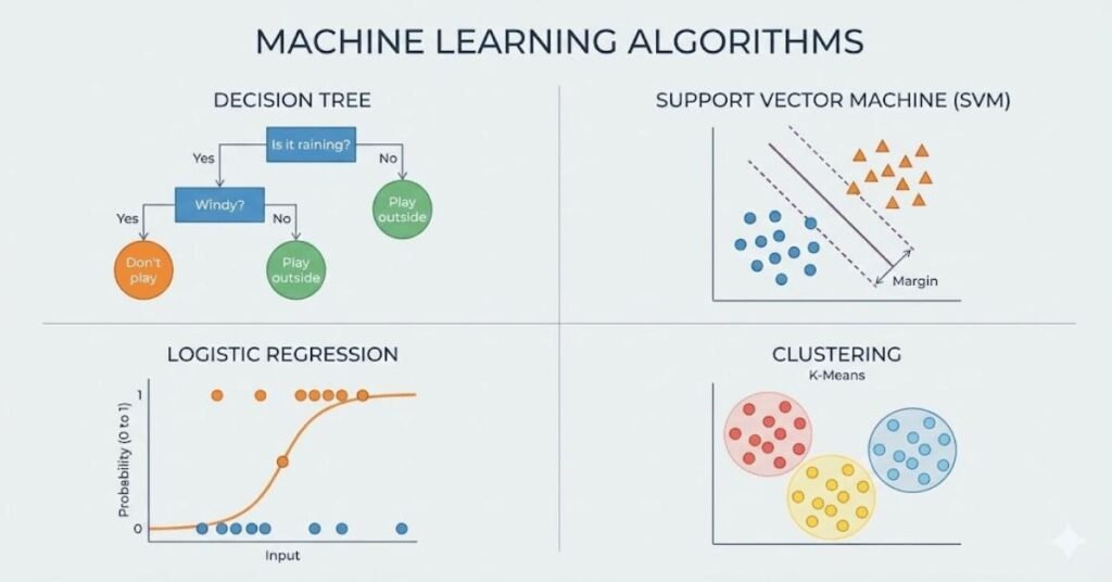
Chapter 10: Decision Trees
10.1 Decision Tree Fundamentals
Q256. What is a decision tree?
A decision tree is a flowchart-like model that makes predictions by asking a series of questions about features. Starting at the root, each node asks a yes-no question about a feature. Based on the answer, you follow the appropriate branch to another node or a leaf. Leaves contain predictions. For example, a tree for spam detection might ask if the email contains certain words, leading to further questions until reaching a leaf that says spam or not spam. Trees are intuitive, interpretable, and handle non-linear relationships naturally.
Q257. What are nodes, branches, and leaves in decision trees?
The root node is the top of the tree representing the entire dataset. Internal nodes represent decision points, asking questions about features and splitting data based on answers. Branches are connections between nodes representing possible answers to questions. Leaf nodes are endpoints containing predictions for examples reaching them. The path from root to leaf represents a sequence of decisions. Trees can be shallow with few levels or deep with many levels. Deeper trees can capture more complex patterns but risk overfitting.
Q258. How does a decision tree make predictions?
For a new example, start at the root and answer each node’s question based on the example’s feature values. Follow the corresponding branch to the next node. Repeat until reaching a leaf. The leaf’s prediction becomes the prediction for that example. For classification, the leaf typically predicts the majority class of training examples that reached it. For regression, it predicts their mean value. Different examples follow different paths, so different rules apply to different regions of feature space.
Q259. Why are decision trees easy to interpret?
Decision trees mirror human decision-making with explicit if-then rules. You can trace exactly why a prediction was made by following the tree path. Visualizing trees shows the logic graphically. Non-technical stakeholders can understand tree decisions. This interpretability is valuable in domains like medicine or finance where understanding model reasoning is crucial. Unlike black-box models, trees provide transparency. However, very deep trees with hundreds of nodes become difficult to interpret despite theoretical interpretability.
Q260. What types of features can decision trees handle?
Decision trees naturally handle both numerical and categorical features without preprocessing. For numerical features, splits are threshold-based like age greater than 30. For categorical features, splits are subset-based like color in red, blue. Trees don’t require feature scaling because splits are based on ordering, not magnitude. They handle missing values by creating special branches. They can capture feature interactions automatically without manually creating interaction terms. This flexibility makes trees versatile and easy to use.
10.2 Training Decision Trees
Q261. How does the CART algorithm work?
Classification and Regression Trees or CART is the standard algorithm for building decision trees. It works top-down, starting with all data at the root. For each node, it considers all possible splits on all features and chooses the split that best separates classes for classification or reduces variance for regression. The data splits into subsets, creating child nodes. The algorithm recursively repeats this process on each child until stopping criteria are met, like reaching maximum depth or minimum samples per node.
Q262. How does the algorithm choose the best split?
For each feature, the algorithm tries all possible split points. For numerical features, it sorts values and tries midpoints between adjacent values. For categorical features, it tries different subset combinations. For each potential split, it calculates a quality measure like Gini impurity or information gain. The split with the best quality score is chosen. This greedy approach considers only the immediate benefit of each split, not long-term consequences. Despite being greedy, it works well in practice.
Q263. What is Gini impurity?
Gini impurity measures how mixed the classes are in a node. It equals the probability of incorrectly classifying a randomly chosen example if you randomly assign a class according to class distribution in that node. Pure nodes with one class have Gini of zero. Maximally mixed nodes with equal classes have higher Gini. Lower Gini is better. The algorithm seeks splits that reduce weighted average Gini of child nodes compared to parent. Gini is computationally efficient and works well in practice.
Q264. What is entropy and information gain?
Entropy measures disorder or uncertainty in a node based on class distribution. Pure nodes have zero entropy, while mixed nodes have higher entropy. Information gain is the reduction in entropy from parent to children after a split. Larger information gain means the split better separates classes. Information gain is an alternative to Gini impurity for choosing splits. Both typically produce similar trees, though Gini is slightly faster to compute. Entropy has theoretical connections to information theory.
Q265. For regression, how are splits chosen?
Regression trees minimize variance rather than impurity. For each potential split, calculate the mean squared error or variance of target values in each child node. Choose the split minimizing the weighted average variance. Leaves predict the mean target value of training examples reaching them. The goal is creating homogeneous regions where target values are similar. This approach naturally handles non-linear relationships because different regions can have different mean predictions.
10.3 Visualizing Decision Trees
Q266. How do you visualize decision trees?
Scikit-learn provides tools for visualizing trees. The plot_tree function creates graphical representations showing nodes, splits, and class distributions. The export_graphviz function exports tree structure to dot format for rendering with Graphviz. Visualization shows the full tree structure with node questions, sample counts, value distributions, and predictions. For small trees, this provides complete insight into model logic. For large trees, visualization helps understand tree structure even if details are overwhelming.
Q267. What information appears in tree visualizations?
Each node in visualizations shows the split condition like sepal length less than or equal to 5.5, the Gini or entropy value, the number of samples reaching that node, the distribution of classes, and for leaves, the predicted class. Colors often indicate class purity, with darker colors showing more homogeneous nodes. This information reveals what the tree learned, which features matter, and how data flows through the tree. It aids debugging and understanding model behavior.
Q268. How can visualization help improve models?
Visualization reveals problems like overfitting when trees are excessively deep with leaves containing single examples. You see which features the tree uses and which it ignores, guiding feature engineering. Unusual splits might indicate data quality issues. Balanced versus unbalanced tree structures show whether complexity is appropriate. If the tree uses many splits on one feature, that feature might need transformation. Visualization makes the abstract concept of model learning concrete and actionable.
Q269. What are the limitations of tree visualization?
Large trees with hundreds or thousands of nodes are impossible to visualize meaningfully. Even moderately deep trees become cluttered and hard to read. Visualization doesn’t scale to ensemble methods like random forests with hundreds of trees. For production models, visualization is rarely used, though it’s valuable during development. Text-based tree representations might be more practical than graphical ones for deep trees, showing the most important splits.
Q270. How does tree depth affect visualization?
Shallow trees with few levels are easy to visualize and understand completely. As depth increases, visualizations become complex and harder to interpret. Beyond depth 5 or 10, full visualization often provides limited insight. For deep trees, focus on visualizing the top levels showing the most important splits, or use text summaries. During model development, intentionally limiting depth creates interpretable trees, balancing performance against understandability.
Chapter 11: Random Forests and Ensemble Methods
11.1 Ensemble Learning Concepts
Q271. What is ensemble learning?
Ensemble learning combines predictions from multiple models to produce better results than any single model. The idea is that different models make different errors, and by aggregating their predictions, errors can cancel out while correct predictions reinforce each other. Think of it like asking multiple experts for opinions then taking a vote or average. Ensemble methods consistently win machine learning competitions and work well in production because they’re more robust and accurate than individual models. They’re a cornerstone of modern machine learning practice.
Q272. Why do ensembles work better than single models?
Ensembles work because individual models have different strengths and weaknesses. One model might excel on certain patterns while another handles different patterns better. By combining them, you get the best of both worlds. Individual models make mistakes, but these mistakes are often different. Averaging or voting across models reduces the impact of any one model’s errors. This principle is similar to why diverse teams make better decisions than individuals. The key is having models that are reasonably accurate but make different types of errors.
Q273. What are the main types of ensemble methods?
The three main ensemble approaches are bagging, boosting, and stacking. Bagging trains multiple models independently on different subsets of data then averages predictions, reducing variance. Boosting trains models sequentially where each model tries to correct errors made by previous ones, reducing bias. Stacking trains diverse models then uses another model to learn how best to combine their predictions. Each approach has different strengths and is suited to different problems. Understanding when to use each is important for practical machine learning.
Q274. What is model diversity and why does it matter?
Model diversity means ensemble members make different types of errors. If all models are identical, combining them provides no benefit since they all make the same mistakes. Diversity comes from using different algorithms, different training data subsets, different feature sets, or different hyperparameters. The more diverse the models while maintaining reasonable accuracy, the better the ensemble performs. Creating diversity while avoiding poor individual models is the art of ensemble building. Too much diversity with low-accuracy models hurts rather than helps.
Q275. How many models should you include in an ensemble?
The optimal number depends on your specific problem and computational constraints. More models generally improve performance up to a point, then gains diminish. For bagging methods like random forests, hundreds of trees are common. For boosting, anywhere from 50 to several hundred models works well. Returns diminish as you add more, and computational cost grows linearly. Start with moderate numbers like 100 and increase if performance improves and resources allow. Monitor validation performance to see when adding more models stops helping.
11.2 Voting Classifiers
Q276. What is a voting classifier?
A voting classifier combines predictions from multiple classification models using voting. For hard voting, each model predicts a class, and the majority vote wins. For soft voting, models output class probabilities, these probabilities are averaged, and the class with highest average probability is selected. Soft voting typically performs better when models provide well-calibrated probabilities. Voting classifiers are the simplest ensemble method, easy to implement and understand. They work best when base models are diverse and reasonably accurate.
Q277. What is the difference between hard and soft voting?
Hard voting treats all model predictions equally, simply counting votes for each class and choosing the majority. Each model gets one vote regardless of confidence. Soft voting weights votes by probability, so a model very confident in its prediction contributes more than an uncertain model. Soft voting uses richer information and typically performs better but requires models that output meaningful probabilities. Hard voting works with any classifier including those that only output class labels. Choose soft voting when your models provide good probability estimates.
Q278. How do you choose models for a voting ensemble?
Select models that are individually accurate but diverse in their approaches. Combining similar models provides little benefit. Good combinations might include a decision tree, a support vector machine, and a neural network since they use fundamentally different approaches. Avoid including weak models just for diversity as they degrade performance. Test different combinations using cross-validation to see what works best for your data. The goal is models that are strong individually but make different types of errors.
Q279. Can you weight votes differently?
Yes, you can assign different weights to different models based on their performance. If one model is clearly stronger, give it more influence by assigning a higher weight. Weights can be determined by validation set performance, with better models receiving higher weights. This weighted voting combines diverse models while appropriately valuing their individual contributions. However, if model quality varies dramatically, it might be better to exclude weak models entirely rather than include them with low weights. Experiment to find what works best.
Q280. What are the computational costs of voting ensembles?
Training cost equals the sum of training all individual models. For most algorithms, this is the dominant cost. Prediction requires running all models and combining results, which is slower than a single model but often acceptable. The computational cost grows linearly with the number of models. If individual models are fast like decision trees, the ensemble remains fast. If individual models are slow like deep neural networks, the ensemble becomes expensive. Parallel training and prediction can help since models are independent.
11.3 Bagging and Pasting
Q281. What is bagging?
Bagging, short for bootstrap aggregating, trains multiple models on different random subsets of the training data created through sampling with replacement. Each model sees a slightly different dataset, creating diversity. Predictions are combined by averaging for regression or voting for classification. Bagging reduces variance because averaging multiple estimates is more stable than any single estimate. It works particularly well with high-variance models like deep decision trees. Bagging is simple, effective, and parallelizable since models train independently.
Q282. What is bootstrap sampling?
Bootstrap sampling creates new datasets by randomly sampling from the original dataset with replacement. Each new dataset has the same size as the original but contains different examples. Some examples appear multiple times, while others don’t appear at all. On average, each bootstrap sample contains about 63 percent unique examples from the original data. This sampling creates the data diversity that makes bagging work. Bootstrap sampling is also used for statistical inference and estimating confidence intervals.
Q283. What is the difference between bagging and pasting?
Bagging samples with replacement, meaning the same example can appear multiple times in a training set. Pasting samples without replacement, so each example appears at most once per training set but different subsets contain different examples. Both create diverse training sets, but bagging’s sampling with replacement typically provides more diversity. Bagging is more commonly used and generally performs slightly better. Both reduce variance and can be parallelized. The choice is usually bagging unless you have specific reasons to prefer pasting.
Q284. Why does bagging reduce variance?
Bagging reduces variance through averaging. Individual models have high variance, meaning their predictions vary significantly with different training data. By training multiple models on different data subsets and averaging their predictions, the random fluctuations tend to cancel out while the systematic patterns remain. Mathematically, the variance of an average of independent random variables is lower than the variance of individual variables. This is why bagging works best with high-variance models like deep trees that overfit.
Q285. Can bagging improve simple models?
Bagging helps most with high-variance models that are prone to overfitting. For low-variance models like linear regression or shallow decision trees, bagging provides minimal benefit because these models are already stable. You won’t hurt performance by bagging simple models, but you’ll add computational cost for little gain. Bagging’s sweet spot is with complex models that individually overfit but collectively generalize well. If your base model underfits, bagging multiple underfitting models still produces an underfitting ensemble.
11.4 Out-of-Bag Evaluation
Q286. What is out-of-bag evaluation?
Out-of-bag evaluation uses data not sampled for each model’s training as a validation set. Since bootstrap sampling includes only about 63 percent of examples per sample, the remaining 37 percent are out-of-bag for that model. Each model can be evaluated on its out-of-bag examples. Aggregating across all models gives an overall performance estimate without needing a separate validation set. This is computationally efficient and maximizes training data usage. Out-of-bag evaluation is a key advantage of bagging.
Q287. How accurate is out-of-bag evaluation?
Out-of-bag evaluation provides performance estimates comparable to cross-validation but with much less computation. Since each example is out-of-bag for multiple models, you get robust predictions. Studies show out-of-bag estimates are reliable for assessing generalization performance. However, they can be slightly optimistic compared to truly independent test sets. For model development and comparison, out-of-bag evaluation works great. For final performance reporting, use a held-out test set. The efficiency makes out-of-bag evaluation very practical.
Q288. Can you use out-of-bag for hyperparameter tuning?
Yes, out-of-bag evaluation can replace cross-validation for tuning hyperparameters like number of trees or tree depth in random forests. Train models with different hyperparameters and compare their out-of-bag scores. This is much faster than cross-validation since you only train once per configuration rather than k times. The efficiency is particularly valuable for large datasets or expensive models. Out-of-bag tuning works well in practice and is widely used for bagging-based algorithms.
Q289. What are the limitations of out-of-bag evaluation?
Out-of-bag evaluation only works with bagging methods that sample with replacement. It doesn’t apply to other ensemble methods like boosting or stacking. The evaluation is slightly optimistic compared to independent test data. With very small datasets, the out-of-bag sets might be too small for reliable estimates. Despite these limitations, out-of-bag evaluation is extremely useful for bagging methods and is one of their key practical advantages.
Q290. How do you interpret out-of-bag scores?
Interpret out-of-bag scores the same way as validation scores. Higher accuracy, F1, or other metrics indicate better performance. Compare out-of-bag scores across different model configurations to select the best. Monitor how scores change with ensemble size to determine when more models stop helping. Out-of-bag scores estimate how the model will perform on new data. If out-of-bag performance is poor, the ensemble won’t generalize well. If it’s good, you can be reasonably confident in deployment.
11.5 Random Forests
Q291. What is a random forest?
A random forest is an ensemble of decision trees trained using bagging with an additional twist: at each split, only a random subset of features is considered. This extra randomness creates more diverse trees that work better together. Random forests are among the most popular and powerful machine learning algorithms, working well across many problems with minimal tuning. They handle non-linear relationships, feature interactions, and mixed data types naturally. Random forests are often the first algorithm to try after simple baselines.
Q292. How does feature randomness help random forests?
Without feature randomness, all trees in a bagged ensemble would be similar because strong features would dominate early splits. Feature randomness ensures different trees use different features, creating true diversity. If one feature is very strong, some trees won’t use it and will discover patterns involving other features. This diversity makes the ensemble more robust. The optimal number of random features to consider per split is typically the square root of total features for classification and one-third for regression.
Q293. How many features should you consider per split?
The standard recommendation is square root of total features for classification and one-third of features for regression. For example, with 100 features, consider 10 for classification or 33 for regression. These are starting points; you can tune this hyperparameter. More features per split gives trees more choices, potentially better individual trees but less diversity. Fewer features increase diversity but might prevent trees from finding good splits. Cross-validation helps find the optimal value for your specific problem.
Q294. How do random forests handle overfitting?
Random forests resist overfitting through multiple mechanisms. Individual trees are high-variance but averaging many trees reduces overall variance. Feature randomness prevents the ensemble from relying too heavily on any single strong feature. You can control tree depth and leaf size to prevent individual trees from overfitting too severely. The combination of these factors makes random forests remarkably resistant to overfitting. You can often use default parameters and get good results without extensive tuning.
Q295. What are the disadvantages of random forests?
Random forests are less interpretable than single decision trees since you can’t easily visualize hundreds of trees. They require more memory and computation than single models. Prediction is slower than simple models though still fast enough for most applications. Training can be slow with very large datasets though parallelization helps. Despite these limitations, random forests are excellent general-purpose algorithms that work well across diverse problems with minimal tuning effort.
11.6 Extra Trees and Feature Importance
Q296. What are extra trees?
Extra trees or extremely randomized trees are like random forests but with even more randomness. Instead of searching for the best split among random features, extra trees select splits completely randomly. This additional randomness creates more diversity and trains faster since finding optimal splits is expensive. Paradoxically, this extra randomness often works as well or better than random forests. Extra trees are worth trying if random forests work well for your problem. They’re faster to train and sometimes more accurate.
Q297. How do you calculate feature importance?
Feature importance measures how much each feature contributes to predictions. For tree-based models, importance is calculated by summing how much each feature reduces impurity across all splits where it’s used, weighted by the number of samples affected. Features used in many splits affecting many samples have high importance. Averaging across all trees gives overall feature importance. These scores help you understand what drives predictions and identify which features to focus on or discard.
Q298. How do you interpret feature importance scores?
Higher scores mean features are more important for predictions. Compare relative scores rather than absolute values. The most important features should make sense given your domain knowledge. If unexpected features rank highly, investigate whether they contain valuable information or are causing problems like data leakage. Very low importance features might be noise that could be removed. Feature importance helps with feature selection and model interpretation. However, correlated features can have importance split between them arbitrarily.
Q299. What are the limitations of feature importance?
Feature importance can be misleading with correlated features since importance gets distributed among them unpredictably. It doesn’t tell you the direction of effects, only magnitude. Importance can be biased toward high-cardinality categorical features. It doesn’t distinguish between features important because they’re predictive versus important because they interact with other features. Despite these limitations, feature importance provides valuable insights and is widely used. Use it as one tool among several for understanding your model.
Q300. Can you use feature importance for feature selection?
Yes, feature importance can guide feature selection. Remove features with very low importance and retrain to see if performance is maintained with fewer features. This reduces complexity and training time. However, be careful not to remove too aggressively as features might interact or provide small but cumulative benefits. Use cross-validation to ensure removed features truly don’t hurt performance. Iterative removal and evaluation finds the minimal feature set maintaining good performance.
11.7 Boosting Methods
Q301. What is boosting?
Boosting trains models sequentially where each model tries to correct errors made by previous models. Unlike bagging where models train independently, boosting models are interdependent. Early models are simple, and subsequent models focus on examples the ensemble struggles with. Predictions are combined through weighted voting. Boosting reduces both bias and variance, often achieving excellent performance. Popular boosting algorithms include AdaBoost, Gradient Boosting, and XGBoost. Boosting is powerful but requires careful tuning to avoid overfitting.
Q302. How does boosting differ from bagging?
Bagging trains models independently in parallel on different data subsets and averages predictions to reduce variance. Boosting trains models sequentially where each focuses on correcting previous errors, reducing both bias and variance. Bagging works best with high-variance models like deep trees. Boosting works with weak learners like shallow trees. Bagging is more parallelizable and harder to overfit. Boosting can achieve higher accuracy but requires more careful tuning. Both are powerful techniques with different strengths.
Q303. What is AdaBoost?
AdaBoost or Adaptive Boosting trains a sequence of weak classifiers, typically shallow decision trees. After each model, it increases weights on misclassified examples so the next model focuses more on them. Final predictions combine all models weighted by their accuracy. AdaBoost was one of the first successful boosting algorithms and remains popular. It works well for binary classification with clean data. However, it’s sensitive to noise and outliers since it heavily focuses on difficult examples which might just be mislabeled.
Q304. What is gradient boosting?
Gradient boosting builds an ensemble by adding models that predict the residual errors of the current ensemble. Each new model is fit to the negative gradient of the loss function, hence the name. This framework is more flexible than AdaBoost, working with different loss functions and supporting regression naturally. Modern implementations like XGBoost, LightGBM, and CatBoost dominate machine learning competitions. Gradient boosting achieves state-of-the-art performance on many structured data problems but requires careful hyperparameter tuning.
Q305. What hyperparameters are important for boosting?
Key hyperparameters include number of models, learning rate, and individual model complexity. More models generally improve performance but increase overfitting risk and training time. Learning rate controls how much each model contributes; smaller rates require more models but often generalize better. Model complexity like tree depth balances bias and variance; boosting typically uses shallow trees. Regularization parameters control overfitting. Tuning these requires cross-validation. Start with conservative values like 100 models, 0.1 learning rate, and depth 3 trees.
11.8 Stacking Methods
Q306. What is stacking?
Stacking or stacked generalization trains a meta-model to combine predictions from multiple base models. Unlike voting which uses simple rules, stacking learns the optimal combination. Base models make predictions on validation data, these predictions become features for the meta-model which learns to combine them optimally. Stacking can achieve excellent performance by leveraging diverse models effectively. However, it’s more complex to implement and tune than simpler ensemble methods. Stacking often appears in competition-winning solutions.
Q307. How do you implement stacking?
Split data into training and validation sets. Train diverse base models on the training set. Use these models to make predictions on the validation set. These predictions become features for the meta-model. Train the meta-model on validation predictions to predict actual targets. For test data, base models make predictions which the meta-model combines. Use cross-validation to generate out-of-fold predictions for the entire training set, avoiding information leakage. The meta-model learns which base models to trust for different scenarios.
Q308. What models work well as base models?
Use diverse models with different strengths as base models. Good combinations include decision trees, linear models, support vector machines, and neural networks. Diversity is crucial; similar models provide redundant information. Each model should be reasonably accurate individually. Poor models hurt the ensemble even if the meta-model tries to weight them down. Five to ten diverse base models typically work well. More models increase complexity without proportional benefit. Focus on diversity over quantity.
Q309. What should you use as a meta-model?
The meta-model should be relatively simple to avoid overfitting. Linear regression or logistic regression work well and are interpretable, showing which base models contribute most. Ridge or Lasso regression add regularization. Simple neural networks or gradient boosting can work but risk overfitting to base model quirks. The meta-model has fewer training examples than base models since it trains on validation predictions, so complexity must be limited. Start simple and add complexity only if validation performance improves.
Q310. What are the challenges with stacking?
Stacking is complex to implement correctly, requiring careful data splitting to avoid leakage. It’s computationally expensive since you train multiple base models plus a meta-model. Overfitting is a risk if the meta-model is too complex or if proper cross-validation isn’t used. Deployment is more complicated since you need to maintain multiple models. Despite these challenges, stacking achieves excellent performance and is worth the effort for high-stakes applications. For most problems, simpler ensembles like random forests or gradient boosting suffice.
Chapter 12: Unsupervised Learning Techniques
12.1 Clustering Fundamentals
Q311. What problems does clustering solve?
Clustering discovers natural groupings in data without predefined labels. It’s useful for customer segmentation where you group customers by behavior to target marketing. Image segmentation groups similar pixels to identify objects. Document clustering organizes articles by topic. Anomaly detection flags points that don’t fit any cluster. Data exploration reveals structure you didn’t know existed. Clustering reduces complexity by working with groups rather than individuals. It’s fundamental for understanding data structure when you don’t have labels.
Q312. How do you evaluate clustering quality?
Without true labels, evaluating clustering is challenging. Internal metrics like silhouette score measure how well points fit their assigned clusters versus other clusters. Higher silhouette scores indicate better-defined clusters. Elbow method plots metric values versus number of clusters; the elbow indicates optimal cluster count. Visual inspection of clusters in reduced dimensions shows whether groupings make sense. If you have domain knowledge, check whether clusters align with meaningful categories. With ground truth labels, use external metrics like adjusted rand index.
Q313. How do you choose the number of clusters?
The elbow method plots total within-cluster variance versus cluster count; the elbow where improvement slows suggests the optimal number. Silhouette analysis shows which cluster counts produce well-separated clusters. Domain knowledge often suggests natural groupings. Cross-validation with downstream tasks shows which cluster count improves overall pipeline performance. Try multiple values and examine results. There’s rarely one correct answer; the best choice depends on your goals. Start with domain-informed guesses then explore nearby values.
Q314. What distance metrics are used in clustering?
Euclidean distance measures straight-line distance between points, the most common choice. Manhattan distance sums absolute differences along each dimension, less sensitive to outliers. Cosine similarity measures angle between vectors, useful for high-dimensional sparse data like text. Correlation distance captures pattern similarity regardless of scale. The right metric depends on your data characteristics. For continuous features on similar scales, Euclidean works well. For sparse high-dimensional data, cosine is better. Distance choice significantly affects results.
Q315. What are hard clustering versus soft clustering?
Hard clustering assigns each point to exactly one cluster. Algorithms like K-means produce hard assignments. Soft clustering or fuzzy clustering assigns membership probabilities to multiple clusters. Points can partially belong to several clusters. Algorithms like fuzzy C-means and Gaussian mixture models produce soft assignments. Soft clustering reflects reality better when boundaries between groups are fuzzy. Hard clustering is simpler and easier to interpret. Choose based on whether your data naturally has overlapping categories or distinct groups.
12.2 K-Means Algorithm
Q316. How does K-means clustering work?
K-means partitions data into K clusters by minimizing within-cluster variance. Start by randomly initializing K cluster centers called centroids. Assign each point to its nearest centroid. Recalculate centroids as the mean of points assigned to them. Repeat assignment and update steps until centroids stop moving significantly. The algorithm is simple, fast, and widely used. It works well for compact, spherical clusters. K-means scales to large datasets efficiently. However, you must specify K upfront and initialization affects results.
Q317. How do you initialize K-means?
Random initialization selects K points randomly as initial centroids. This is simple but can lead to poor results. K-means plus plus initialization chooses centroids spread far apart, typically producing better results. It selects the first centroid randomly, then chooses subsequent centroids with probability proportional to their squared distance from nearest existing centroid. This spreads initial centroids across the data. Most implementations use K-means plus plus by default. Running K-means multiple times with different initializations and keeping the best result helps avoid bad local minima.
Q318. Why is K-means sensitive to initialization?
K-means is a greedy algorithm that can get stuck in local minima depending on initialization. If initial centroids are poorly placed, the algorithm might converge to a suboptimal clustering. Different initializations can produce different final clusters with different quality. K-means plus plus initialization mitigates this but doesn’t eliminate it completely. Running the algorithm multiple times with different random seeds and selecting the clustering with lowest total within-cluster variance helps find better solutions. Modern implementations do this automatically.
Q319. How do you choose K for K-means?
Use the elbow method by plotting total within-cluster sum of squares versus K. As K increases, variance decreases but with diminishing returns. The elbow where the curve bends suggests optimal K. Silhouette analysis shows which K values produce well-separated clusters. Try values suggested by domain knowledge. Use clustering as preprocessing for supervised learning and choose K that maximizes downstream task performance. There’s no universal answer; the best K depends on your data and goals. Start with educated guesses then experiment.
Q320. What are K-means limitations?
K-means assumes clusters are spherical and equally sized, failing with elongated or irregular shapes. It’s sensitive to outliers since means are affected by extreme values. You must specify K upfront without knowing the true number of clusters. Different runs can produce different results due to initialization. K-means struggles with clusters of very different densities. Despite limitations, K-means works well for many practical problems and is often the first clustering algorithm to try. For complex cluster shapes, consider alternatives like DBSCAN or hierarchical clustering.
12.3 DBSCAN Algorithm
Q321. What is DBSCAN?
DBSCAN stands for Density-Based Spatial Clustering of Applications with Noise. It groups points in high-density regions while labeling sparse points as outliers. Unlike K-means, DBSCAN doesn’t require specifying the number of clusters upfront. It discovers clusters of arbitrary shapes. Points with many neighbors within a radius epsilon are core points. Points reachable from core points belong to clusters. Points not reachable are outliers. DBSCAN excels at finding clusters with irregular shapes and handling noise naturally.
Q322. What parameters does DBSCAN require?
DBSCAN requires two parameters. Epsilon defines the radius around each point to search for neighbors. Min_samples sets the minimum number of neighbors for a point to be considered a core point. These parameters control what’s considered a dense region. Larger epsilon connects more points into clusters. Smaller epsilon creates tighter clusters. Higher min_samples requires denser regions. Choosing these parameters requires understanding your data scale and density. Try multiple values and examine results. Domain knowledge helps determine appropriate neighborhood sizes.
Q323. How does DBSCAN handle outliers?
DBSCAN explicitly identifies outliers as points not belonging to any cluster. Points in low-density regions not reachable from core points are labeled as noise. This makes DBSCAN robust to outliers unlike K-means where outliers distort cluster centers. The outliers detected might represent anomalies, noise, or genuinely distinct points. You can examine them separately or remove them. This outlier detection capability is valuable for data cleaning and anomaly detection applications.
Q324. When should you use DBSCAN versus K-means?
Use K-means for spherical clusters of similar size when you know the number of clusters. Use DBSCAN when clusters have irregular shapes, varying densities, or when you don’t know K upfront. DBSCAN handles outliers better. K-means is faster for large datasets. DBSCAN works in high dimensions but parameter tuning becomes harder. For exploratory analysis without prior knowledge, try DBSCAN first. For production systems with clean data and known cluster counts, K-means is simpler. Both have their place depending on problem characteristics.
Q325. What are DBSCAN limitations?
DBSCAN struggles with clusters of varying densities since one epsilon can’t capture them all. In high dimensions, density becomes less meaningful due to the curse of dimensionality. Parameter selection is not intuitive and requires experimentation. Computational complexity is higher than K-means though various optimizations help. DBSCAN doesn’t work well with very high-dimensional data. Despite limitations, it’s powerful for appropriate problems, particularly those with irregular cluster shapes or significant noise.
Chapter 13: Introduction to Neural Networks with Keras
13.1 Neural Network Basics
Q326. What is an artificial neural network?
An artificial neural network is a computing system inspired by biological brains. It consists of layers of interconnected nodes called neurons. Each connection has a weight that gets adjusted during training. Neurons receive inputs, multiply them by weights, sum them up, add a bias, then apply an activation function. This simple computation repeated across thousands or millions of neurons creates powerful models that learn complex patterns. Neural networks excel at image recognition, natural language processing, and many other tasks where patterns are intricate and difficult to program explicitly.
Q327. What is a perceptron?
The perceptron is the simplest neural network, a single neuron that takes inputs, multiplies each by a weight, sums them with a bias, and applies an activation function to produce an output. It learns by adjusting weights based on errors. The perceptron can learn linear decision boundaries, separating classes with a straight line or hyperplane. Despite its simplicity, the perceptron is historically important as the foundation of modern neural networks. It illustrates core concepts like weighted sums, activation functions, and learning through error correction that scale to deep networks.
Q328. What are layers in neural networks?
Neural networks organize neurons into layers. The input layer receives data, with one neuron per feature. Hidden layers sit between input and output, transforming data through learned representations. The output layer produces final predictions, with neurons for each class in classification or a single neuron for regression. Deep networks have multiple hidden layers, enabling them to learn hierarchical features. Information flows forward through layers during prediction. During training, errors flow backward to adjust weights. Layer architecture determines network capacity and behavior.
Q329. What is a fully connected layer?
A fully connected or dense layer connects every neuron to every neuron in the previous layer. If the previous layer has 100 neurons and the current layer has 50, there are 5,000 connections. Each connection has a learnable weight. Fully connected layers can learn arbitrary relationships but require many parameters. They’re standard in traditional neural networks. Modern architectures often use specialized layers like convolutional or recurrent layers that have fewer parameters and encode useful inductive biases for specific data types.
Q330. What is forward propagation?
Forward propagation is the process of computing predictions by passing data through the network layer by layer. Input data enters the network, each layer computes weighted sums and applies activation functions, producing outputs that become inputs for the next layer. This continues until reaching the output layer which produces final predictions. Forward propagation is straightforward computation flowing in one direction. Understanding it is essential since it defines what the network computes. Training involves repeatedly performing forward propagation to get predictions, computing loss, then backpropagation to update weights.
13.2 Activation Functions
Q331. What is an activation function?
An activation function applies a non-linear transformation to a neuron’s weighted sum of inputs. Without activation functions, multiple layers would collapse to a single linear transformation, no more powerful than linear regression. Activation functions introduce non-linearity, enabling networks to learn complex patterns. Common choices include ReLU, sigmoid, and tanh. Different activation functions have different properties affecting training speed and final performance. Choosing appropriate activation functions for different layers is important for network design.
Q332. What is the ReLU activation function?
ReLU stands for Rectified Linear Unit. It outputs the input if positive, otherwise zero. Mathematically it’s max of zero and x. ReLU is simple, fast to compute, and doesn’t saturate for positive values. It’s become the default activation function for hidden layers because it works well in practice. Networks with ReLU train faster than with sigmoid or tanh. However, ReLU neurons can die, always outputting zero if they receive consistently negative inputs. Variants like Leaky ReLU address this by allowing small negative outputs.
Q333. When should you use sigmoid activation?
Sigmoid squashes inputs to values between zero and one, making it useful for binary classification output layers where you need probabilities. It was commonly used in hidden layers historically but is now mostly replaced by ReLU. Sigmoid saturates for large positive or negative inputs, meaning gradients approach zero. This causes vanishing gradient problems in deep networks, slowing training. Use sigmoid for binary classification outputs but prefer ReLU for hidden layers unless you have specific reasons to use sigmoid.
Q334. What is the tanh activation function?
Tanh or hyperbolic tangent squashes inputs to values between negative one and positive one, centered at zero. It’s similar to sigmoid but zero-centered, which can help training. Tanh was popular for hidden layers before ReLU became dominant. Like sigmoid, tanh saturates for extreme inputs causing vanishing gradients. It’s still occasionally used in recurrent networks. For feedforward hidden layers, ReLU usually works better. Understanding tanh is important for reading older papers and understanding activation function evolution.
Q335. What is the softmax activation function?
Softmax converts a vector of numbers into probabilities that sum to one. It’s used in multi-class classification output layers. For each class, softmax exponentiates its score then divides by the sum of all exponentiated scores. This ensures outputs are positive and sum to one, interpretable as probabilities. The class with the highest score gets the highest probability. Softmax is differentiable, allowing backpropagation. It’s the standard choice for multi-class classification outputs. For binary classification, sigmoid is simpler though softmax also works.
13.3 Backpropagation
Q336. What is backpropagation?
Backpropagation is the algorithm for training neural networks by computing gradients of the loss with respect to every weight. It works backward through the network using the chain rule of calculus. After forward propagation produces a prediction and loss, backpropagation computes how much each weight contributed to that loss. These gradients tell you how to adjust weights to reduce loss. Without backpropagation, training deep networks would be impossible. Understanding backpropagation conceptually helps you design better architectures and diagnose training problems even though frameworks compute gradients automatically.
Q337. How does the chain rule apply to backpropagation?
The chain rule allows computing derivatives of composite functions by multiplying derivatives of each component. In neural networks, the loss depends on the final layer output, which depends on the previous layer, and so on. The chain rule lets you decompose this into manageable pieces. To find how loss changes with respect to an early layer’s weights, multiply the derivative of loss with respect to final output, times the derivative of final output with respect to previous layer, and so on backward. This chain of multiplications gives you gradients for all weights.
Q338. Why is backpropagation efficient?
Backpropagation computes gradients for all weights with one backward pass. Naively, you might think you need to recompute the forward pass for each weight to see how perturbing it changes the loss, which would be impossibly expensive. Backpropagation cleverly reuses intermediate computations. The backward pass takes similar time to the forward pass. This efficiency makes training networks with millions of parameters feasible. Modern deep learning frameworks implement automatic differentiation, computing gradients automatically for arbitrary network architectures using generalized backpropagation.
Q339. What are vanishing and exploding gradients?
Vanishing gradients occur when gradients become extremely small as they propagate backward through many layers. This happens with activation functions like sigmoid that saturate. Weights barely update, and early layers don’t learn. Deep networks trained poorly before solutions like ReLU and better initialization. Exploding gradients are the opposite, where gradients grow exponentially large. This causes massive parameter updates and training instability. Gradient clipping limits gradient magnitude to prevent explosions. Modern architectures and techniques largely solve these problems, enabling training very deep networks.
Q340. How do you diagnose gradient flow problems?
Monitor gradient magnitudes during training. If gradients are consistently near zero for early layers, you have vanishing gradients. If gradients spike to huge values, you have explosions. Plot gradient distributions to visualize flow. Check whether loss decreases; if not, gradients might not flow properly. Use gradient checking during development to verify backpropagation implementation is correct. Modern frameworks and techniques make gradient problems less common, but understanding them helps when training doesn’t work as expected.
13.4 Building Models with Keras
Q341. What is Keras?
Keras is a high-level neural network API running on top of TensorFlow. It provides a user-friendly interface for building and training models with much less code than raw TensorFlow. Keras emphasizes ease of use, allowing rapid prototyping. It supports both simple sequential models and complex multi-input, multi-output models. Keras became TensorFlow’s official high-level API, making it the standard way most people build neural networks with TensorFlow. Learning Keras is essential for practical deep learning.
Q342. How do you create a sequential model?
The Sequential model is the simplest Keras API for linear stacks of layers. Create a Sequential instance then add layers one by one with the add method. Specify each layer’s size and activation function. For example, add a Dense layer with 64 neurons and ReLU activation, then another Dense layer with 10 neurons and softmax for classification. After adding all layers, compile the model specifying optimizer, loss function, and metrics. This simple API works for most straightforward architectures.
Q343. What does model compilation do?
Compilation configures the model for training. You specify the optimizer like Adam or SGD that controls how weights update. You specify the loss function like categorical crossentropy for multi-class classification or mean squared error for regression. You specify metrics to monitor like accuracy. Compilation doesn’t train the model but prepares it for training. After compilation, you can call fit to train on data. Compilation parameters significantly affect training behavior and final performance.
Q344. How do you train a Keras model?
Call the fit method with training data, labels, batch size, and number of epochs. Optionally provide validation data to monitor generalization during training. The model trains for the specified epochs, updating weights to minimize loss. Fit returns a history object containing loss and metric values per epoch, useful for plotting training curves. You can use callbacks during training for behaviors like early stopping or learning rate adjustment. Training is straightforward but choosing good hyperparameters requires experimentation.
Q345. How do you make predictions with a trained model?
Call the predict method with new data. For classification, it returns probability distributions over classes. Call predict_classes for class labels directly. For regression, predict returns numerical predictions. You can predict on single examples or batches. Predictions are fast, often real-time even for complex models. For production, you can save trained models and load them later to make predictions without retraining. Keras makes the entire process from building to training to prediction streamlined and intuitive.
13.5 Model Architecture Design
Q346. How do you choose the number of hidden layers?
Start simple with one or two hidden layers and add more if validation performance improves. More layers enable learning more complex features but risk overfitting and slow training. For simple problems, shallow networks suffice. For complex problems like image recognition, deep networks with dozens of layers work better. Use validation performance as your guide. Modern architectures for computer vision might have 50+ layers, while tabular data models often use just 2-3 hidden layers. Problem complexity and data availability determine optimal depth.
Q347. How do you choose layer sizes?
Common practice is to use similar sizes across layers or gradually decrease size toward outputs. Start with moderate sizes like 64 or 128 neurons. Larger layers increase capacity but require more data and risk overfitting. Smaller layers limit capacity, potentially underfitting. Try a few sizes and use validation performance to decide. Modern practice often uses fixed sizes across many layers rather than tapering. Total parameter count matters more than individual layer sizes. Balance between model capacity and available data.
Q348. What is the functional API?
The functional API provides more flexibility than Sequential, supporting complex architectures with multiple inputs, multiple outputs, or non-linear connections. You create input layers, connect them through transformations, and specify outputs explicitly. This enables branching networks, skip connections, and shared layers. The functional API is more verbose but necessary for advanced architectures. It’s the standard approach for research and complex production systems. Learning it opens up the full power of Keras beyond simple sequential models.
Q349. How do you create models with multiple inputs?
With the functional API, create separate Input layers for each input source. Process each input through its own layers, then concatenate or otherwise combine them. Continue processing the combined representation through shared layers to outputs. This architecture allows learning from heterogeneous data like images plus metadata. Each input can have its own specialized preprocessing layers before combination. Multiple inputs are common in production systems handling diverse data sources.
Q350. What are skip connections?
Skip connections directly connect earlier layers to later layers, bypassing intermediate layers. The later layer receives both the skip connection and normal input. Skip connections help gradients flow backward, enabling much deeper networks. They allow later layers to access both low-level and high-level features. ResNet popularized skip connections, enabling networks with hundreds of layers. They’re now standard in many architectures. Implementing skip connections requires the functional API since they create non-sequential connectivity patterns.
🧩 Boost Your ML Hands-On Skills with 50+ How-to Guides — Practice Now →
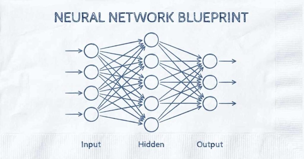
2. 50 Self-Preparation Prompts Using ChatGPT
How to Use These Prompts Effectively
These prompts are designed to help you prepare for machine learning and deep learning interviews using ChatGPT or similar AI assistants. Each prompt is crafted to deepen your understanding of specific concepts in a conversational, accessible way. Copy these prompts directly into ChatGPT, then engage in follow-up questions to clarify anything you don’t understand. Treat this as having a personal tutor available 24/7 to help you master machine learning concepts.
Section 1: Understanding Core Concepts
Prompt 1: Machine Learning Fundamentals
“Explain machine learning to me as if I’m a complete beginner with no technical background. Use everyday examples like cooking or shopping to illustrate how machines learn from data. Then gradually introduce technical terms, explaining each one simply. Help me understand the difference between traditional programming and machine learning.”
Prompt 2: Supervised vs Unsupervised Learning
“Compare supervised and unsupervised learning using real-world scenarios. Give me three examples of each type from different industries like healthcare, retail, and entertainment. Explain why each problem requires that specific learning approach. Then quiz me with five scenarios and ask me to identify whether they need supervised or unsupervised learning.”
Prompt 3: Bias-Variance Tradeoff
“Break down the bias-variance tradeoff concept using a simple analogy like target practice or baking cookies. Explain what happens when bias is too high, when variance is too high, and how to find the sweet spot. Show me how this relates to underfitting and overfitting with visual descriptions I can imagine.”
Prompt 4: Overfitting Explained
“Explain overfitting using the analogy of memorizing versus understanding. Give me warning signs that my model is overfitting and practical techniques to prevent it. Walk me through a scenario where a student preparing for exams either memorizes answers or truly understands concepts, relating this to model training.”
Prompt 5: Training, Validation, and Test Sets
“Guide me through why we need three separate datasets for machine learning. Use an analogy of a student taking practice tests, mock exams, and final exams. Explain what happens if I use the same data for training and testing, and why this is a critical mistake in machine learning projects.”
Section 2: Data Handling and Preprocessing
Prompt 6: Handling Missing Data
“Walk me through all the different strategies for handling missing data in a dataset. Explain when to use deletion, mean imputation, median imputation, forward fill, and advanced methods. Give me a decision tree or flowchart in words that helps me choose the right strategy based on how much data is missing and why it’s missing.”
Prompt 7: Feature Scaling Techniques
“Explain the difference between normalization and standardization in simple terms. When should I use each one? Give me examples of algorithms that require feature scaling and those that don’t. Show me step-by-step calculations for both methods using a simple example with three numbers.”
Prompt 8: Data Cleaning Strategies
“Describe a complete data cleaning workflow from start to finish. Include checking for duplicates, handling outliers, fixing data types, dealing with inconsistent formatting, and validating data quality. Give me a checklist I can use for every machine learning project to ensure my data is clean before modeling.”
Prompt 9: Feature Engineering
“Teach me about feature engineering using practical examples. Show me how to create new features from existing ones, including polynomial features, interaction terms, date-time features, and text features. Give me five creative feature engineering ideas for a house price prediction problem.”
Prompt 10: Dealing with Imbalanced Data
“Explain the problem of imbalanced datasets where one class has much more data than another. Walk me through techniques like oversampling, undersampling, SMOTE, and class weights. Use a fraud detection scenario with 99% legitimate transactions and 1% fraud to illustrate each technique.”
Section 3: Algorithm Deep Dives
Prompt 11: Decision Trees Simplified
“Explain how decision trees make predictions using a simple example like deciding whether to play tennis based on weather conditions. Walk me through how the tree is built, how it chooses which questions to ask, and how it knows when to stop splitting. Make it visual and intuitive.”
Prompt 12: Random Forests Explained
“Describe random forests using the wisdom of crowds analogy. Explain why many slightly different decision trees together make better predictions than one perfect tree. Walk me through the two sources of randomness in random forests: bootstrap sampling and feature randomness. Help me understand when to use random forests versus single decision trees.”
Prompt 13: Support Vector Machines
“Teach me about Support Vector Machines using the concept of finding the widest road between two cities. Explain margin, support vectors, and the kernel trick in simple terms. Show me when SVMs work well and when they struggle. Use a visual description of how SVM draws decision boundaries.”
Prompt 14: K-Means Clustering
“Guide me through the K-means algorithm step by step using an example of grouping customers into segments. Explain how it starts, how it updates, and how it decides to stop. Then explain the challenges: choosing K, dealing with outliers, and understanding when K-means is the right choice.”
Prompt 15: Linear and Logistic Regression
“Explain the difference between linear regression and logistic regression using simple examples. Show me when to use each one, how they make predictions differently, and why logistic regression is called regression but used for classification. Walk me through the math in the simplest possible way.”
Section 4: Model Evaluation
Prompt 16: Confusion Matrix Mastery
“Break down the confusion matrix for me. Explain true positives, false positives, true negatives, and false negatives using a medical diagnosis example. Then show me how to calculate accuracy, precision, recall, and F1-score from the confusion matrix. Give me practice scenarios to test my understanding.”
Prompt 17: Precision vs Recall Tradeoff
“Help me understand when to optimize for precision versus recall using real-world examples like spam detection, disease screening, and fraud detection. Explain the tradeoff between these metrics and how changing the decision threshold affects both. Quiz me on scenarios asking which metric matters more.”
Prompt 18: ROC Curve Interpretation
“Explain ROC curves and AUC scores in simple language. What does it mean when AUC is 0.5 versus 0.9 versus 1.0? How do I interpret different points on the ROC curve? Use a visual description to help me understand what the curve is showing about my classifier’s performance.”
Prompt 19: Cross-Validation Techniques
“Teach me about different cross-validation methods: k-fold, stratified k-fold, leave-one-out, and time series cross-validation. When should I use each one? Walk me through why cross-validation is better than a single train-test split. Give me practical advice on choosing the right CV strategy.”
Prompt 20: Evaluation Metrics for Regression
“Explain MAE, MSE, RMSE, and R-squared for regression problems. What’s the difference between these metrics and when should I use each one? How do I interpret R-squared values? Give me examples showing when one metric might look good while another reveals problems with my model.”
Section 5: Deep Learning Concepts
Prompt 21: Neural Networks for Beginners
“Explain neural networks from scratch as if I’ve never heard of them. Use the analogy of how our brain processes information. Walk me through neurons, layers, weights, biases, and activation functions. Make it so simple that I could explain it to my grandmother.”
Prompt 22: Activation Functions Compared
“Compare different activation functions: ReLU, sigmoid, tanh, and softmax. Explain what each one does, when to use it, and why. Use graphs described in words to help me visualize their shapes. Tell me which activation functions to use for hidden layers versus output layers.”
Prompt 23: Backpropagation Demystified
“Explain backpropagation without heavy math. Use the analogy of a company identifying which departments need improvement after poor quarterly results. How does the network figure out which weights to adjust? Walk me through the concept of gradients flowing backward through the network.”
Prompt 24: Convolutional Neural Networks
“Teach me about CNNs for image recognition. Explain what convolution means using simple examples like applying Instagram filters. What are filters, kernels, pooling, and feature maps? Help me understand why CNNs work better for images than regular neural networks.”
Prompt 25: Recurrent Neural Networks
“Explain RNNs and why they’re good for sequential data like text or time series. Use an analogy of reading a book where understanding depends on previous sentences. What are LSTM and GRU? Why do vanilla RNNs struggle with long sequences? Make it intuitive and easy to remember.”
Section 6: Practical Implementation
Prompt 26: Building Your First Neural Network
“Guide me through building a simple neural network from scratch using Keras. Explain each step: importing libraries, preparing data, defining layers, compiling the model, training, and evaluating. Give me working code with detailed comments explaining what each line does and why.”
Prompt 27: Classification Project Workflow
“Walk me through a complete classification project from start to finish. Include exploratory data analysis, preprocessing, feature engineering, model selection, training, evaluation, and interpretation. Give me a checklist of steps I should never skip, even under time pressure.”
Prompt 28: Hyperparameter Tuning Guide
“Explain hyperparameter tuning strategies. What’s the difference between grid search, random search, and Bayesian optimization? Which hyperparameters should I tune first for different algorithms? Give me a practical workflow for tuning a random forest and a neural network.”
Prompt 29: Model Deployment Basics
“Teach me about deploying machine learning models to production. What considerations are different from just building accurate models? Explain model serialization, API creation, monitoring, and maintenance. Give me a simple roadmap from trained model to deployed application.”
Prompt 30: Feature Selection Methods
“Explain different feature selection techniques: filter methods, wrapper methods, and embedded methods. When should I remove features? Walk me through using feature importance, correlation analysis, and recursive feature elimination. How do I know if I’ve removed too many features?”
Section 7: Advanced Topics
Prompt 31: Ensemble Learning Strategies
“Break down ensemble learning: bagging, boosting, and stacking. Why do multiple models together outperform single models? Explain random forests, gradient boosting, and XGBoost in simple terms. Give me rules of thumb for when to use ensemble methods.”
Prompt 32: Regularization Techniques
“Explain L1 regularization, L2 regularization, dropout, and early stopping. Why does adding penalties help models generalize better? How do I choose regularization strength? Walk me through a scenario where regularization saves a model from overfitting.”
Prompt 33: Dimensionality Reduction
“Teach me about PCA (Principal Component Analysis) using simple examples. Why do we need dimensionality reduction? Explain the difference between PCA and t-SNE. When would I use each one? Help me understand how to choose the number of components to keep.”
Prompt 34: Transfer Learning Applications
“Explain transfer learning using the analogy of how learning to play piano helps with learning organ. When is transfer learning useful? Walk me through taking a pre-trained image model and fine-tuning it for my specific classification task. What layers should I freeze versus retrain?”
Prompt 35: Reinforcement Learning Basics
“Introduce me to reinforcement learning using examples like training a dog or learning to play video games. Explain agents, environments, actions, rewards, and policies. How is this different from supervised learning? Give me real-world applications where RL excels.”
Section 8: TensorFlow and Keras
Prompt 36: TensorFlow Fundamentals
“Explain TensorFlow basics for someone new to deep learning frameworks. What are tensors? How does TensorFlow differ from NumPy? Walk me through creating tensors, performing operations, and understanding the computational graph. Keep it practical and example-driven.”
Prompt 37: Keras Sequential vs Functional API
“Compare Keras Sequential API and Functional API. When should I use each one? Show me code examples of building the same network using both approaches. Explain how to create models with multiple inputs, multiple outputs, and skip connections using the Functional API.”
Prompt 38: Custom Layers and Models
“Teach me how to create custom layers and models in Keras. When do I need custom components versus using built-in layers? Walk me through building a custom activation function and a custom layer with learnable parameters. Explain the structure of custom models.”
Prompt 39: Callbacks in Keras
“Explain Keras callbacks and why they’re useful. Walk me through EarlyStopping, ModelCheckpoint, ReduceLROnPlateau, and TensorBoard callbacks. Give me practical examples of when to use each one and how to configure them for best results during training.”
Prompt 40: Saving and Loading Models
“Guide me through different ways to save and load Keras models. What’s the difference between saving the entire model versus just weights? How do I save model architecture separately? Explain best practices for model versioning and deployment.”
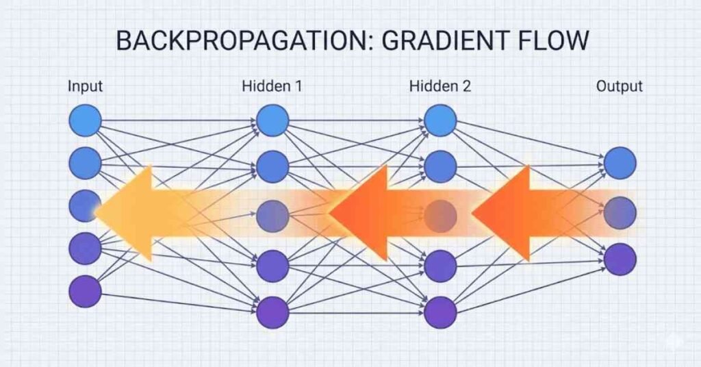
Section 9: Optimization Techniques
Prompt 41: Gradient Descent Variations
“Explain the differences between batch gradient descent, stochastic gradient descent, and mini-batch gradient descent. Why is mini-batch the most commonly used? Walk me through the tradeoffs in convergence speed, stability, and computational efficiency. How do I choose batch size?”
Prompt 42: Advanced Optimizers
“Compare Adam, RMSprop, AdaGrad, and SGD with momentum. How does each optimizer work and when should I use which one? Explain adaptive learning rates in simple terms. Give me a decision tree for choosing the right optimizer for different problems.”
Prompt 43: Learning Rate Scheduling
“Teach me about learning rate schedules. Why start with large learning rates and decrease over time? Explain step decay, exponential decay, and cyclical learning rates. How do I implement learning rate scheduling in Keras? When is it worth the extra complexity?”
Prompt 44: Batch Normalization Explained
“Explain batch normalization and why it helps neural networks train faster and better. How does it work? Where should I add batch normalization layers in my network? Walk me through the benefits and potential downsides. Use intuitive explanations rather than complex math.”
Prompt 45: Gradient Clipping
“Explain the exploding gradient problem and how gradient clipping solves it. When do I need gradient clipping? How do I choose the clipping threshold? Walk me through implementing gradient clipping in practice and monitoring whether it’s helping or hurting training.”
Section 10: Generative AI and LLMs
Prompt 46: Large Language Models Overview
“Explain how large language models like GPT work in simple terms. What is a transformer architecture? How do these models understand and generate text? Walk me through the training process and why they need massive amounts of data. Make it accessible to someone without deep NLP background.”
Prompt 47: Prompt Engineering Fundamentals
“Teach me prompt engineering best practices. How do I write prompts that get better responses from language models? Explain few-shot learning, chain-of-thought prompting, and prompt templates. Give me examples of poorly written versus well-written prompts and explain the differences.”
Prompt 48: Embeddings and Vector Stores
“Explain word embeddings and vector databases. How do words become numbers that capture meaning? What are vector stores used for in AI applications? Walk me through how semantic search works using embeddings. Use simple analogies to explain these concepts.”
Prompt 49: RAG Architecture
“Explain Retrieval Augmented Generation (RAG) systems. Why combine retrieval with generation? Walk me through the components: document chunking, embedding, vector search, and context injection. How does RAG solve the problem of LLMs not knowing recent information? Give me a practical use case.”
Prompt 50: Fine-tuning Large Language Models
“Teach me about fine-tuning pre-trained language models for specific tasks. What’s the difference between fine-tuning and training from scratch? Explain parameter-efficient fine-tuning methods like LoRA. When should I fine-tune versus use prompt engineering? What resources do I need?”
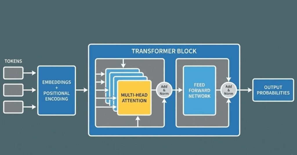
How to Maximize Learning from These Prompts
Best Practices
- One Prompt at a Time: Don’t rush through all 50 prompts in one day. Take time to truly understand each concept before moving to the next.
- Ask Follow-Up Questions: When ChatGPT explains something, ask “Can you give me another example?” or “What if I change this parameter?” to deepen understanding.
- Request Practice Problems: After learning a concept, ask “Give me 5 practice questions to test my understanding of this concept.”
- Relate to Real Projects: Ask “How would I use this concept in a real-world project like predicting customer churn?”
- Create Study Notes: After each prompt session, summarize what you learned in your own words. This reinforces learning.
- Test Your Explanations: Try explaining the concept to someone else or write it down as if teaching a beginner.
Additional Learning Strategies
- Visual Learning: Ask ChatGPT to describe concepts visually when you’re confused: “Can you describe what this would look like as a diagram?”
- Code Examples: Request working code: “Show me Python code that implements this concept with detailed comments.”
- Common Mistakes: Ask “What are the most common mistakes beginners make with this concept?”
- Interview Angles: Request “What interview questions might test this concept and how should I answer them?”
- Connect Concepts: Ask “How does this concept relate to the previous topics I’ve learned?”
Creating Your Own Prompts
As you progress, create custom prompts based on your weak areas:
- “I struggle with understanding [concept]. Explain it using [specific analogy related to my background].”
- “Compare [concept A] and [concept B] side by side with pros, cons, and when to use each.”
- “Give me a real interview scenario where I’d need to apply [concept] and walk me through the answer.”
Final Tips for Interview Success
Use these prompts over several weeks, not all at once. Space out your learning for better retention. Combine this ChatGPT learning with hands-on coding practice. Build small projects applying each concept you learn. The combination of theoretical understanding from these prompts and practical coding experience will prepare you thoroughly for machine learning and deep learning interviews.
Remember, the goal isn’t just to memorize answers but to develop genuine understanding that lets you explain concepts clearly and apply them to new problems. These prompts are your starting point for deeper exploration. Good luck with your interview preparation!
✨ Follow Your ML & Deep Learning Learning Path — Beginner to Advanced →
3.Communication Skills and Behavioural Interview Preparation
Introduction to Behavioral Interviews
Technical skills alone won’t land you a machine learning job. Employers want to know if you can communicate complex ideas clearly, work well with teams, handle pressure, and fit into their company culture. This section prepares you for the behavioral and communication aspects of ML/DL interviews that often determine whether you receive an offer.
Chapter 1: Professional Communication Skills
1.1 Effective Technical Communication
Why Technical Communication Matters
As a machine learning professional, you’ll need to explain complex algorithms to non-technical stakeholders, write clear documentation, present findings to executives, and collaborate with cross-functional teams. Your ability to translate technical jargon into business value determines your career growth.
Key Principles of Technical Communication
Start with the conclusion or main point before diving into details. Your audience wants to know the outcome first. Use the pyramid principle where you present the key message, then supporting arguments, then detailed evidence. This structure keeps people engaged.
Avoid jargon when speaking to non-technical audiences. Instead of saying “our convolutional neural network achieved 94% accuracy on the validation set,” say “our AI model correctly identifies products 94 times out of 100, which will reduce manual inspection costs by half.”
Use analogies to explain complex concepts. Compare neural networks to how children learn from examples. Describe gradient descent as finding the lowest point in a valley while blindfolded. These mental pictures make abstract ideas concrete.
Practice Exercise
Explain one of these concepts to a non-technical friend or family member: overfitting, cross-validation, or ensemble learning. Ask them to repeat back what they understood. Refine your explanation based on their feedback.
1.2 Explaining Complex Concepts Simply
The Layered Explanation Approach
Use three layers when explaining technical concepts. Start with the simplest one-sentence summary. If they want more, provide a paragraph with key details. If they’re still interested, dive into technical specifics.
For example, explaining a recommendation system:
- Layer 1: “We built a system that suggests products customers might like based on their past purchases.”
- Layer 2: “The system looks at patterns in what customers bought together and finds similar customers to make personalized suggestions.”
- Layer 3: “We use collaborative filtering with matrix factorization, specifically an SVD approach, combined with content-based filtering using item embeddings trained on product descriptions.”
Real-World Examples Always Win
Connect abstract concepts to everyday experiences. When explaining clustering, mention how Netflix groups similar shows together. When discussing classification, reference email spam filters everyone uses. These connections make technical concepts relatable.
Handling “I Don’t Know” Gracefully
When asked something you don’t know, be honest but show your problem-solving approach. Say “I haven’t worked with that specific technique, but based on my understanding of similar methods, I would approach it by…” This demonstrates intellectual honesty and analytical thinking.
1.3 Active Listening Skills
The Power of Listening in Interviews
Many candidates fail interviews not because they lack knowledge but because they don’t listen carefully to questions. Interviewers notice when you answer a different question than what was asked. Active listening shows respect and professionalism.
Listen for Intent, Not Just Words
When an interviewer asks “Tell me about a challenging project,” they’re really asking about your problem-solving ability, perseverance, and learning mindset. When they ask “How do you handle conflicts,” they want to assess your emotional intelligence and teamwork skills.
Techniques for Better Listening
Pause for two seconds before answering to process the question fully. If a question is unclear, ask for clarification rather than guessing. Paraphrase complex questions back to confirm understanding: “So you’re asking how I would handle a situation where model performance drops in production?”
Take brief notes during technical discussions. This shows engagement and helps you remember key points for follow-up questions. It also gives you a moment to think.
1.4 Body Language and Non-Verbal Communication
Your Body Speaks Before You Do
In video or in-person interviews, non-verbal cues communicate confidence, enthusiasm, and professionalism. Sit up straight but relaxed. Maintain eye contact without staring. Smile naturally when greeting and during casual conversation.
Video Interview Specific Tips
Position your camera at eye level to create natural eye contact. Look at the camera when speaking, not at the screen showing your face. Ensure good lighting on your face. Test your setup beforehand. Dress professionally even for remote interviews as it affects your mindset.
Nervous Habits to Avoid
Don’t fidget with pens, tap fingers, or play with hair. These signal nervousness and distract from your message. Instead, use purposeful hand gestures when explaining concepts. Keep hands visible but relaxed. Plant your feet firmly to ground yourself physically and mentally.
Reading Interviewer Signals
Notice when interviewers lean forward with interest or sit back looking satisfied. If they glance at their watch or seem distracted, wrap up your point concisely. If they nod encouragingly, you’re on the right track. Adjust your communication style based on these cues.
1.5 Email and Professional Writing
Crafting Professional Emails
Write clear subject lines that summarize content: “Follow-up on ML Engineer Interview” or “Question about Model Deployment Process.” Start emails with appropriate greetings and end with professional signatures including your contact information.
Keep emails concise. Busy hiring managers appreciate brevity. Use bullet points for multiple items. Bold or underline key information sparingly. Proofread before sending to catch typos that undermine professionalism.
Thank You Notes After Interviews
Send personalized thank you emails within 24 hours of each interview. Reference specific topics discussed to show attentiveness. Express genuine enthusiasm about the role and company. Mention something you learned during the interview that excites you. These notes reinforce positive impressions.
Documentation Skills
Good documentation is crucial for ML projects. Practice writing clear README files for your GitHub projects. Explain what the project does, how to install and run it, and any important considerations. Include example usage. This demonstrates your ability to create production-quality work.
1.6 Presentation Skills for Technical Audiences
Structuring Technical Presentations
Begin with context and business problem before diving into technical details. Executives care about impact, not implementation specifics. Technical peers want methodology details. Tailor content to your audience.
Use visuals effectively. Include charts showing model performance improvements, architecture diagrams, and results visualizations. Avoid slides packed with text. One key idea per slide with supporting visuals works best.
Handling Questions During Presentations
Welcome questions as they show engagement. If asked something complex, acknowledge it and offer to discuss details after the presentation. If you don’t know the answer, promise to follow up with information later. Never fake knowledge as experts will catch you.
Practice Makes Perfect
Record yourself presenting technical content and watch the playback. Notice filler words like “um” and “like.” Check your pacing, clarity, and enthusiasm. Present to friends or colleagues for feedback. Join Toastmasters or similar groups to build confidence.
Chapter 2: Common Behavioral Interview Questions
2.1 Tell Me About Yourself
Structure Your Response
This question opens most interviews. Prepare a compelling 2-3 minute summary covering your background, relevant experience, key achievements, and why you’re interested in this specific role. Don’t recite your resume; tell a story.
Sample Framework
Start with your current or most recent role and key accomplishments. “I’m currently a data scientist at XYZ Company where I built recommendation systems that increased user engagement by 35%.”
Move to relevant background. “Before that, I completed my degree in Computer Science and worked on several ML projects including image classification and NLP applications.”
Conclude with motivation. “I’m particularly excited about this role because of your work in healthcare AI. Combining machine learning with meaningful social impact aligns perfectly with my career goals.”
What to Avoid
Don’t share your entire life story starting from childhood. Don’t focus on unrelated jobs or hobbies unless they demonstrate transferable skills. Don’t be overly modest or overly boastful. Strike a confident, authentic tone.
Practice Exercise
Write out your “tell me about yourself” answer. Time it to ensure it’s under 3 minutes. Practice until you can deliver it naturally without memorization. Record yourself to check for filler words and nervous habits.
2.2 Why Machine Learning and Deep Learning
Demonstrate Genuine Passion
Interviewers want to know if you’re truly passionate about ML or just chasing trendy job titles. Share your origin story. What first fascinated you about machine learning? Was it a specific project, course, or problem you encountered?
Connect Personal Interest to Impact
Explain why ML excites you beyond just being intellectually interesting. Perhaps you’re driven by solving real-world problems, the creativity involved in modeling, or the rapid pace of innovation. Connect your interest to tangible outcomes.
Example Response
“I became passionate about machine learning during my undergraduate studies when I built a model to predict student dropout rates. Seeing how data-driven insights could directly improve educational outcomes was powerful. The combination of mathematics, programming, and real-world impact drew me to specialize in this field. I particularly enjoy deep learning because of the creative problem-solving involved in architecture design and the ability to tackle previously unsolvable problems like image recognition.”
2.3 Your Strengths and Weaknesses
Choosing Relevant Strengths
Select strengths directly relevant to ML roles: analytical thinking, attention to detail, quick learning, persistence in debugging, ability to explain technical concepts, or collaborative skills. Support each strength with specific examples.
Instead of just saying “I’m detail-oriented,” say “I’m meticulous about data quality and validation. In my last project, I discovered a subtle data leakage issue during preprocessing that would have inflated our model’s performance by 10%. Catching this early prevented deploying a flawed model.”
Addressing Weaknesses Authentically
Choose real weaknesses that aren’t deal-breakers, then explain how you’re addressing them. Good examples include public speaking anxiety you’re overcoming through practice, initial unfamiliarity with a specific tool you’re now learning, or tendency toward perfectionism that you’re balancing with pragmatic deadlines.
Avoid cliché weaknesses like “I work too hard” that sound insincere. Also avoid critical weaknesses like “I struggle with basic math” for an ML role.
Sample Weakness Response
“Earlier in my career, I focused heavily on model accuracy and sometimes spent too much time optimizing for marginal improvements. I’ve learned to balance perfection with practical constraints. Now I establish clear success criteria upfront and know when good enough is sufficient, especially for prototypes. This helps me deliver value faster while maintaining quality.”
2.4 Career Goals and Aspirations
Align Goals with Company Direction
Research the company before interviews. Understand their technology stack, business challenges, and future direction. Frame your goals to align with opportunities the company offers.
If they’re expanding into computer vision, express interest in specializing there. If they value technical leadership, mention aspirations to lead ML teams eventually. Show that growing with this company advances your career.
Balance Ambition with Realism
Express ambitious but realistic goals. “In five years, I see myself as a senior ML engineer leading complex projects and mentoring junior team members” is better than “I want to be VP of AI in two years.”
Show you’ve thought about growth paths. Mention interest in both deepening technical expertise and developing leadership skills. This demonstrates maturity and long-term thinking.
Sample Response
“My immediate goal is to become highly proficient in production ML systems, understanding the full lifecycle from experimentation to deployment and monitoring. I’m particularly interested in your MLOps practices and would love to contribute to improving them. Long-term, I’d like to lead ML projects that combine technical innovation with clear business impact. I’m drawn to this role because it offers both hands-on technical work and opportunities to collaborate across functions, which aligns perfectly with my growth trajectory.”
2.5 Why This Company
Do Your Homework
Research the company thoroughly. Understand their products, recent news, company culture, technical challenges, and competitive position. Follow their engineering blog if available. Check employee reviews on Glassdoor.
Identify 2-3 specific reasons you’re excited about this company beyond just “it’s a great company.” Maybe they’re solving interesting technical problems, have impressive ML talent, offer great learning opportunities, or align with your values.
Avoid Generic Answers
Don’t say “You’re a leader in the industry” or “Great company culture” without specifics. These apply to many companies and show you haven’t done research. Instead, reference specific projects, technologies, or initiatives that excite you.
Example Response
“I’m excited about this opportunity for three main reasons. First, your work on real-time fraud detection at scale involves fascinating technical challenges around model latency and adversarial robustness that I’d love to tackle. Second, I was impressed by your recent blog post on model explainability for regulatory compliance, showing you balance innovation with responsibility. Finally, your culture of knowledge sharing through meetups and open-source contributions aligns with my belief in collaborative learning. I want to work somewhere I can grow while contributing to meaningful problems.”
2.6 Salary Expectations Discussion
Researching Market Rates
Before interviews, research typical salaries for ML roles in your location and experience level. Use resources like Glassdoor, Levels.fyi, Payscale, and LinkedIn Salary. Factor in company size, industry, and your specific skills.
Handling the Salary Question
If asked early in the process, try to defer: “I’d prefer to learn more about the role and responsibilities before discussing compensation. I’m confident we can reach a fair agreement if we’re a mutual fit.”
If pressed, provide a range based on research: “Based on my research for senior ML engineers in this area with my experience level, I’m targeting the range of X to Y. However, I’m flexible depending on the complete compensation package and growth opportunities.”
Negotiation Mindset
Remember that compensation includes base salary, bonuses, equity, benefits, learning budget, and work-life balance. Consider the total package. It’s appropriate to negotiate professionally. Companies expect it and respect candidates who know their worth.
Chapter 3: Situation-Based Questions
3.1 Handling Difficult Team Members
The STAR Method
Structure situation-based answers using STAR: Situation (context), Task (your responsibility), Action (what you did), Result (outcome). This framework ensures complete, organized responses.
Example Scenario
Situation: “In my last project, I worked with a data engineer who consistently delivered data late, delaying our modeling work.”
Task: “I needed to address this professionally while maintaining our working relationship and meeting project deadlines.”
Action: “I scheduled a one-on-one conversation to understand his challenges. He was overwhelmed with multiple urgent requests. We collaboratively created a prioritization system and clear timelines. I also adjusted my workflow to start with available data while waiting for remaining datasets.”
Result: “Deliveries improved significantly. We built mutual respect and the project launched on time. I learned the importance of understanding teammates’ perspectives before jumping to conclusions.”
Key Lessons to Highlight
Emphasize communication, empathy, problem-solving, and positive outcomes. Show you handle conflicts professionally and constructively rather than letting them fester or escalating unnecessarily.
3.2 Working Under Pressure
Demonstrating Grace Under Fire
Employers want to know you can handle tight deadlines, unexpected problems, and high-stakes situations without panic. Share examples where you maintained quality despite pressure.
Sample Response
“During a product launch, our recommendation model showed unexpected behavior in production just days before release. I immediately assembled the team, systematically debugged by checking data pipeline, feature engineering, and model predictions. We discovered a subtle bug in how timestamps were handled across time zones. I coordinated a fix, thorough testing, and a staggered rollout to verify everything worked. The launch succeeded on schedule. This taught me the importance of comprehensive testing and having rollback plans for production systems.”
What Interviewers Assess
They’re evaluating your prioritization skills, ability to stay calm, technical problem-solving under constraints, communication during crises, and learning from stressful situations. Show you’re resilient and focused.
3.3 Dealing with Project Failures
Honesty About Setbacks
Everyone faces failures. Discussing them authentically shows maturity. Interviewers want to see how you handle disappointment, what you learn, and how you bounce back.
Framing Failure Constructively
Choose a real failure but not a catastrophic one. Explain the situation, acknowledge your role without excessive blame of others, describe lessons learned, and show how you applied those lessons subsequently.
Example Response
“Early in my career, I built a churn prediction model that performed great in validation but failed in production. I was so focused on maximizing accuracy that I overlooked deployment constraints around latency and feature availability. The model relied on features that weren’t available in real-time. This taught me to consider deployment requirements from day one. Now I always involve engineering early in projects and prototype with production-feasible features. My models since then have transitioned to production smoothly.”
Turning Failure into Growth
Emphasize learning and improvement. Show that failures made you better at your craft. Demonstrate humility and willingness to adapt. This honest reflection impresses interviewers more than claiming you never fail.
3.4 Managing Tight Deadlines
Prioritization and Trade-offs
Explain how you manage competing priorities and make smart trade-offs when time is limited. ML projects often face pressure to deliver quickly while maintaining quality.
Strategy Discussion
“When facing tight deadlines, I start by clarifying what’s truly critical versus nice-to-have. I communicate honestly with stakeholders about what’s realistic. I prioritize getting a working baseline model quickly, then iterate improvements. For example, when given two weeks for a project typically needing a month, I delivered a solid but simple model on time, documented limitations, and outlined a roadmap for enhancements. Stakeholders appreciated transparency and the project provided immediate value while we continued improving it.”
3.5 Resolving Conflicts
Conflict Resolution Skills
ML work involves collaboration with diverse teams. Conflicts arise around priorities, approaches, or resources. Show you can navigate disagreements professionally.
Sample Scenario
“I once disagreed with a product manager about which ML problem to tackle first. She wanted a personalization feature for engagement while I felt fraud prevention was more urgent. Rather than arguing, I suggested we evaluate both using a simple impact-effort matrix. We estimated potential business impact, technical complexity, and implementation time for each. The analysis showed fraud prevention had higher immediate impact with similar effort. She agreed to prioritize it. This taught me that data-driven discussions resolve conflicts better than opinions.”
3.6 Adapting to Changes
Flexibility in Fast-Paced Environments
ML and tech move quickly. Requirements change, new tools emerge, and priorities shift. Demonstrate adaptability and positive attitude toward change.
Example Response
“Midway through developing a TensorFlow model, our company standardized on PyTorch. Rather than resisting, I saw it as a learning opportunity. I spent evenings upskilling in PyTorch, translating my work gradually, and actually found several aspects I preferred. The experience made me more versatile. Now I embrace changes in tools or direction as chances to grow rather than obstacles.”
Chapter 4: Technical Leadership Questions
4.1 Leading Machine Learning Projects
Demonstrating Leadership Potential
Even in individual contributor roles, leadership qualities matter. Discuss times you took initiative, influenced technical decisions, or guided others.
Project Leadership Example
“I led a sentiment analysis project for customer reviews. I started by aligning stakeholders on success criteria and timeline. I broke the work into sprints, assigning tasks based on team strengths. I conducted daily standups to track progress and unblock issues. When a junior member struggled with data preprocessing, I paired with him to teach best practices. We delivered two weeks early with 89% accuracy, beating our 85% target. The experience taught me that clear communication and supporting team members are as important as technical skills.”
4.2 Mentoring Junior Team Members
Teaching and Knowledge Sharing
Ability to mentor shows depth of knowledge and leadership readiness. Share examples of helping others grow technically.
Mentorship Example
“I mentored a new graduate joining our team. I created a structured onboarding covering our tech stack, code base, and ML pipeline. I did weekly knowledge-sharing sessions on topics like debugging models and feature engineering. I reviewed his code patiently, explaining not just what to change but why. He became productive quickly and later told me my mentorship shaped his approach to ML engineering. I enjoy teaching and helping others succeed.”
4.3 Making Technical Decisions
Decision-Making Framework
Explain how you evaluate technical trade-offs and make sound decisions, especially when options have pros and cons.
Sample Response
“When choosing between different model architectures, I evaluate multiple factors systematically. For a text classification project, I considered accuracy, training time, inference latency, interpretability, and maintenance burden. I prototyped three approaches: logistic regression, random forest, and LSTM. The LSTM was most accurate but slowest. Given our latency requirements, I recommended random forest which balanced accuracy and speed well. I documented this analysis so future team members understood the rationale. This systematic approach to technical decisions has served me well.”
4.4 Handling Model Failures
Production Issues and Debugging
Discuss how you diagnose and fix production ML issues. This shows operational maturity and technical depth.
Debugging Example
“A recommendation model started returning poor suggestions. I systematically investigated: checked for data pipeline issues, verified feature distributions hadn’t shifted, reviewed recent code changes, and analyzed prediction patterns. I discovered the training data refresh had failed, so the model was stale. I implemented monitoring for data freshness and added alerts to catch similar issues early. This taught me that robust ML systems need comprehensive monitoring, not just model performance tracking.”
4.5 Prioritizing Multiple Projects
Resource Management
Explain how you balance competing demands and allocate time effectively across projects.
Prioritization Strategy
“I use a combination of business impact, urgency, and effort to prioritize. I maintain a project tracker with status and blockers. I communicate proactively when I’m overcommitted rather than letting deliverables slip. For example, when assigned three simultaneous projects, I negotiated timelines with stakeholders, worked on the highest-impact project full-time while delegating portions of others, and delivered everything with clear communication throughout. Transparency about capacity and progress builds trust.”
4.6 Cross-Functional Collaboration
Working Beyond Your Team
ML success requires collaboration with data engineers, product managers, business analysts, and executives. Show you work well across functions.
Collaboration Example
“For a customer churn model, I collaborated extensively with business teams. I met with customer success to understand churn drivers qualitatively. I worked with analysts to identify relevant metrics. I involved product managers in defining success criteria. I presented findings to executives in business terms rather than technical jargon. This cross-functional approach ensured the model addressed real business needs and gained organization-wide buy-in. I learned that technical excellence alone isn’t enough; understanding business context and building relationships are equally critical.”
Chapter 5: Problem-Solving Scenarios
5.1 Debugging Model Performance Issues
Systematic Troubleshooting
Walk through your debugging methodology when models underperform. Show analytical thinking and domain expertise.
Debugging Framework
“When debugging model issues, I follow a checklist. First, verify data quality and check for distribution shifts. Second, review feature engineering for bugs or leakage. Third, examine model architecture and hyperparameters. Fourth, check the training process for issues like underfitting or overfitting. Fifth, validate evaluation metrics align with business goals. For instance, when a fraud detection model had low precision, I discovered class imbalance was causing it to over-predict fraud. Adjusting class weights and the decision threshold fixed this.”
5.2 Handling Data Quality Problems
Real-World Data Challenges
Discuss experience with messy real-world data and how you cleaned and validated it.
Example Scenario
“I once received customer data with 40% missing values, inconsistent formats, and obvious errors like ages over 150. I created a comprehensive cleaning pipeline: imputed missing values using appropriate strategies, standardized formats, removed or corrected outliers based on domain knowledge, and added validation checks. I documented all transformations for reproducibility. I also worked with the data team to improve upstream data collection. Clean data is foundational for good models, so investing time here always pays off.”
5.3 Optimizing Model Training Time
Efficiency and Resource Management
Explain strategies for reducing training time when facing constraints.
Optimization Approach
“To speed up training for a large image dataset, I implemented several optimizations. I used data generators to load batches on-the-fly rather than loading everything into memory. I leveraged GPU acceleration and mixed-precision training. I used transfer learning with a pretrained model instead of training from scratch. I experimented with smaller image resolutions initially to find good hyperparameters quickly. These strategies reduced training time from 12 hours to 2 hours while maintaining accuracy. Resource efficiency is crucial for iterating quickly.”
5.4 Dealing with Imbalanced Datasets
Class Imbalance Solutions
Describe techniques for handling imbalanced data, a common ML challenge.
Practical Example
“For a medical diagnosis problem with 95% negative and 5% positive cases, I addressed imbalance through multiple strategies. I used stratified sampling to maintain class ratios in validation sets. I experimented with oversampling the minority class using SMOTE and undersampling the majority class. I adjusted class weights in the loss function to penalize minority class errors more. I used appropriate metrics like F1-score and AUC rather than accuracy. The combination of these techniques improved minority class recall significantly while maintaining precision.”
5.5 Selecting Appropriate Algorithms
Algorithm Choice Rationale
Explain how you select algorithms for different problems, showing understanding of their strengths and limitations.
Decision Process
“Algorithm selection depends on multiple factors. For structured tabular data with clear feature relationships, I start with gradient boosting or random forests. For image data, CNNs are natural choices. For sequence data, RNNs or transformers work well. I also consider interpretability requirements, training data size, and latency constraints. I typically baseline with simple models first, then increase complexity if needed. For a credit scoring problem, I chose logistic regression over neural networks because interpretability was critical for regulatory compliance and it performed adequately.”
5.6 Managing Computational Resources
Resource Optimization
Discuss managing limited computational resources, especially relevant for resource-constrained environments.
Resource Management Example
“Working with limited GPU resources, I optimized our workflow. I used smaller batch sizes and gradient accumulation to fit models in memory. I scheduled long training jobs overnight. I profiled code to identify bottlenecks and optimized slow operations. I used model compression techniques like quantization for deployment. I also advocated for cloud GPU instances for critical experiments, presenting cost-benefit analysis to management. Smart resource management lets you achieve strong results even with constraints.”
Chapter 6: Project Discussion Preparation
6.1 Presenting Your ML Projects
Project Storytelling Structure
Prepare to discuss 3-5 significant projects in detail. Structure each story with problem, approach, challenges, results, and learnings.
Project Template
Problem: “We needed to predict customer lifetime value to optimize marketing spend.”
Approach: “I built a regression model using historical transaction data, customer demographics, and behavioral features. I experimented with linear regression, random forests, and gradient boosting.”
Challenges: “Data was sparse for new customers. I addressed this with survival analysis techniques and cold-start strategies.”
Results: “The model achieved R-squared of 0.72, improving targeting accuracy by 25% and ROI on marketing campaigns by 18%.”
Learning: “I learned the importance of understanding business metrics deeply. Technical accuracy matters less than business impact.”
6.2 Explaining Technical Challenges
Deep-Diving into Difficulties
Interviewers probe into project challenges to assess problem-solving depth. Prepare to explain technical obstacles in detail.
Example Discussion
“The biggest challenge was catastrophic forgetting in our continual learning system. As we trained on new data, the model forgot previously learned patterns. I researched solutions and implemented elastic weight consolidation to preserve important weights while learning new tasks. I also added experience replay, maintaining a buffer of past examples to periodically retrain. This reduced forgetting by 60% while enabling adaptation to new patterns.”
6.3 Discussing Project Outcomes
Quantifying Impact
Always quantify project results when possible. Numbers demonstrate real impact and business value.
Impact Examples
Instead of “improved model performance,” say “increased accuracy from 78% to 91%, reducing false positives by 40%.”
Instead of “built a recommendation system,” say “built a system serving 2 million users daily, increasing click-through rate by 23% and revenue per user by $1.50.”
Concrete metrics prove your work delivered value. Track impact metrics for all projects to discuss in interviews.
6.4 Describing Your Role and Contributions
Distinguishing Team vs Individual Work
Be honest about your specific contributions in team projects. Interviewers can tell when you’re exaggerating.
Clear Attribution
Say “I was responsible for the data pipeline and feature engineering” rather than “We built a model” if you didn’t personally build the model.
Say “I proposed and implemented the ensemble approach that improved accuracy by 5%” to highlight your specific innovation.
Use “I” for your work and “we” for team efforts. This honesty shows integrity and team player attitude.
6.5 Lessons Learned from Projects
Growth Mindset
Discuss what you learned from each project, including mistakes and how you’d approach similar problems differently now.
Reflection Example
“Looking back, I would have involved business stakeholders earlier in defining success metrics. We built a highly accurate model but discovered later that speed mattered more than perfect accuracy for the use case. Now I start every project by deeply understanding business requirements and constraints, not just technical goals.”
6.6 Future Improvements and Ideas
Forward-Thinking Perspective
Show you think beyond current solutions by discussing potential improvements you didn’t have time to implement.
Enhancement Ideas
“Given more time, I would experiment with transfer learning from related domains to improve performance with limited data. I would also implement better model interpretability tools to help business users trust predictions. Additionally, I’d build more comprehensive A/B testing infrastructure to measure real-world impact more rigorously.”
Chapter 7: Industry Awareness
7.1 Current Trends in Machine Learning
Staying Updated
Demonstrate awareness of current ML trends and their implications. Read papers, follow ML blogs, and attend conferences virtually.
Discussion Points
Talk about large language models and their impact on NLP tasks. Discuss the shift toward MLOps and productionizing models. Mention federated learning for privacy-preserving ML. Reference specific recent developments like GPT-4, Stable Diffusion, or advances in reinforcement learning.
Show you’re not just aware but have thoughtful opinions about these trends and their applications.
7.2 Generative AI Applications
Understanding GenAI Impact
Generative AI is transforming many industries. Show you understand its potential and limitations.
Practical Applications
Discuss how generative AI enables content creation, code generation, drug discovery, and personalized education. Acknowledge challenges like hallucinations, bias, and ethical concerns. Show balanced perspective recognizing both opportunities and risks.
7.3 Ethical Considerations in AI
Responsible AI Practices
Ethics in AI is increasingly important. Show awareness of bias, fairness, transparency, and privacy issues.
Ethical Framework
Discuss fairness in model predictions across demographic groups. Mention the importance of explainable AI for high-stakes decisions. Reference privacy-preserving techniques like differential privacy. Show you consider ethical implications proactively, not as afterthoughts.
Example Discussion
“In developing the hiring prediction model, I was particularly careful about fairness. I checked for disparate impact across gender and ethnicity. I removed potentially biased features and tested the model extensively for discrimination. Even though it meant slightly lower accuracy, ensuring fairness was non-negotiable. AI practitioners have a responsibility to build systems that benefit everyone equitably.”
7.4 Industry Best Practices
Professional Standards
Show familiarity with ML engineering best practices like version control, experiment tracking, code reviews, and documentation.
Best Practices Discussion
“I follow several best practices in my work. I version control everything including data, code, and models using Git and DVC. I track experiments systematically with MLflow to reproduce results. I write comprehensive documentation and tests. I conduct code reviews with peers to catch bugs and share knowledge. These practices ensure my work is reproducible, maintainable, and professional quality.”
7.5 Popular ML Tools and Frameworks
Technical Ecosystem
Demonstrate familiarity with current tools and ability to learn new ones quickly.
Tool Knowledge
Discuss experience with frameworks like TensorFlow, PyTorch, and Scikit-learn. Mention data processing tools like Pandas and Spark. Reference deployment platforms like Docker, Kubernetes, and cloud services. Show you’re pragmatic about tools, choosing based on project needs rather than personal preference.
7.6 Staying Updated with Technology
Continuous Learning Habits
Explain how you keep skills current in a rapidly evolving field.
Learning Strategy
“I stay updated through multiple channels. I follow key researchers on Twitter and read papers from top conferences like NeurIPS and ICML. I complete online courses on new topics. I participate in Kaggle competitions to practice new techniques. I attend local ML meetups and present my work. I contribute to open-source projects. Continuous learning is essential in this field and I make it a priority.”
Chapter 8: Soft Skills Development
8.1 Time Management Techniques
Productivity and Organization
Demonstrate ability to manage time effectively across multiple responsibilities.
Time Management Approach
“I use a combination of techniques. I prioritize tasks by impact and urgency using an Eisenhower matrix. I time-block my calendar, dedicating focused time to deep work on complex problems. I batch similar tasks like code reviews. I use tools like Notion for project tracking and Todoist for task management. I also protect time for learning and staying current with the field.”
8.2 Teamwork and Collaboration
Being a Team Player
ML work is collaborative. Show you work well with others and contribute positively to team culture.
Collaboration Skills
Discuss sharing knowledge through documentation and presentations. Mention helping teammates when they’re stuck. Reference participating actively in code reviews. Show you celebrate team successes and support members during challenges. Demonstrate you value diverse perspectives and create inclusive environments.
8.3 Adaptability and Flexibility
Embracing Change
Technology and business priorities change rapidly. Show you adapt positively.
Adaptability Example
“When our team pivoted from batch predictions to real-time inference, I quickly learned about streaming architectures and low-latency optimization. I refactored my models for efficiency and worked with engineers on deployment. Rather than seeing the change as disruptive, I viewed it as expanding my skill set. Flexibility is crucial in technology.”
8.4 Critical Thinking Skills
Analytical Mindset
Demonstrate ability to think deeply about problems and question assumptions.
Critical Thinking Application
“I don’t accept requirements at face value. I probe to understand underlying business problems. For a request to ‘predict sales,’ I asked what decisions would be made with predictions, what accuracy level was needed, and what timeline was required. This revealed that category-level predictions were sufficient, simpler than the product-level model initially requested. Critical thinking prevents wasted effort on wrong problems.”
8.5 Continuous Learning Mindset
Growth Orientation
Show commitment to continuous improvement and lifelong learning.
Learning Culture
“I view every project as a learning opportunity. I reflect on what went well and what could improve. I seek feedback actively and incorporate it. I’m not afraid to admit knowledge gaps and work to fill them. I believe the best ML practitioners are perpetual students. This growth mindset keeps me excited about the field even after years of practice.”
8.6 Professional Ethics
Integrity and Responsibility
Demonstrate ethical behavior and professional conduct.
Ethical Standards
“I maintain high ethical standards in my work. I’m honest about model limitations and uncertainties. I never manipulate results to look better than they are. I respect data privacy and handle sensitive information carefully. I give credit to others’ ideas and contributions. I speak up when I see concerning practices. Trust and integrity are foundational to professional relationships.”
Final Interview Preparation Tips
Mock Interview Practice
Practice with friends, mentors, or online platforms like Pramp or Interviewing.io. Record yourself to identify areas for improvement. Get comfortable with video interview format.
Company-Specific Research
Study each company’s products, technology stack, recent news, and culture. Tailor your answers to align with their specific needs and values. Prepare company-specific questions to ask interviewers.
Questions to Ask Interviewers
Prepare thoughtful questions showing genuine interest:
- What does success look like in this role in the first 90 days?
- What are the biggest challenges the ML team faces currently?
- How does the team balance research exploration with product delivery?
- What opportunities exist for learning and growth?
- How does the company support work-life balance?
Managing Interview Anxiety
Prepare thoroughly to build confidence. Practice deep breathing before interviews. Remember that interviewers want you to succeed. Focus on conversation rather than interrogation. If you make mistakes, acknowledge and move forward gracefully.
Follow-Up and Reflection
Send thank-you notes within 24 hours. Reflect on each interview to identify improvement areas. Keep a learning journal noting questions asked and how you could answer better. Each interview improves your skills for the next.
💼 Train with Experts & Crack ML/DL Interviews Faster — Enroll Now!
4.ADDITIONAL PREPARATION ELEMENTS
Introduction to Additional Preparation
Technical knowledge and behavioral skills form the foundation of interview success, but several additional elements significantly increase your chances of landing a machine learning role. This section covers practical aspects like building an impressive resume, creating a strong portfolio, optimizing your online presence, and navigating the job search process strategically. These elements often make the difference between getting interviews and being overlooked, or between receiving one offer versus multiple competing offers.
Chapter 1: Resume Building for ML Roles
1.1 Structuring Your ML Resume
The One-Page Rule
For early to mid-career professionals, keep your resume to one page. Recruiters spend an average of six seconds scanning each resume initially. Every word must earn its place. Senior professionals with 10+ years of experience can use two pages, but even then, brevity demonstrates respect for the reader’s time.
Essential Sections in Order
Start with your name and contact information at the top. Include phone number, professional email, LinkedIn URL, and GitHub profile. Next comes a brief professional summary of 2-3 sentences highlighting your ML expertise and key strengths. Follow with work experience in reverse chronological order, then education, technical skills, and finally projects or publications if space permits.
Professional Summary That Captures Attention
Your summary should immediately convey your value proposition. Instead of generic statements like “passionate machine learning engineer seeking opportunities,” write something specific: “Machine Learning Engineer with 3 years building production recommendation systems serving 5M+ users. Expertise in deep learning, NLP, and MLOps with proven track record reducing customer churn by 28%.”
Work Experience: The STAR Format
For each role, include company name, your title, and dates. Then list 3-5 bullet points describing achievements using the STAR format compressed into single powerful statements. Each bullet should start with a strong action verb like developed, implemented, optimized, or designed. Follow with what you did, the technologies used, and the quantified impact.
Example: “Developed real-time fraud detection system using XGBoost and neural networks, processing 50K transactions per second with 94% accuracy, reducing fraud losses by $2.3M annually.”
Education Section
List your degree, institution, graduation year, and relevant coursework or honors. For recent graduates, include GPA if above 3.5. Mention relevant projects, thesis work, or research if applicable. As you gain experience, this section shrinks while work experience expands.
1.2 Highlighting Technical Skills
Organizing Your Tech Stack
Create clear categories for your skills. Use headings like Programming Languages, ML Frameworks, Data Tools, Cloud Platforms, and Databases. This organization helps recruiters and ATS systems quickly identify your qualifications.
Under each category, list technologies in order of proficiency. Don’t claim expertise in tools you’ve barely used. Distinguish between proficient, experienced, and familiar if using a skills matrix.
The Right Level of Detail
For programming languages, specify your proficiency level contextually through your project descriptions rather than rating yourself with stars or percentages, which are subjective. Instead of saying “Python: 4/5 stars,” demonstrate Python expertise through projects listed in your experience.
Keywords for ATS Optimization
Many companies use Applicant Tracking Systems that scan resumes for keywords before human eyes see them. Study job descriptions carefully and incorporate relevant terminology naturally. If the job mentions TensorFlow, PyTorch, computer vision, and model deployment, ensure these terms appear in your resume if you have that experience.
Avoid keyword stuffing, which is obvious and counterproductive. Instead, weave terms naturally into your achievements. “Built computer vision model using PyTorch for object detection” hits multiple keywords naturally.
Balancing Breadth and Depth
Show you have deep expertise in core areas while demonstrating adaptability through experience with various tools. Employers want specialists who can also learn new technologies. Emphasize 2-3 areas where you’re truly expert while showing familiarity with the broader ecosystem.
1.3 Showcasing Projects Effectively
Choosing Which Projects to Include
Select projects that demonstrate skills relevant to the target role. If applying for computer vision positions, prioritize CV projects. Include a mix of personal projects, academic work, and professional experience to show well-rounded capabilities.
Choose projects that tell a story of progression and learning. Show how you’ve tackled increasingly complex problems or applied ML to diverse domains. Diversity demonstrates versatility while depth in specific areas shows expertise.
Project Descriptions That Sell
Each project description should follow this structure: What problem did it solve? What technologies did you use? What was the outcome or impact? Keep descriptions to 1-2 lines on your resume with links to detailed documentation on GitHub or your portfolio site.
Example: “Built sentiment analysis system for product reviews using BERT and PyTorch, achieving 91% accuracy on 100K reviews, deployed via Flask API. GitHub: github.com/yourname/sentiment-analysis“
Quantifying Project Impact
Always include metrics when possible. Dataset size shows you can handle scale. Accuracy or performance metrics demonstrate technical achievement. Processing speed or latency shows production readiness. Cost savings or revenue impact proves business value.
If your project is academic or personal without direct business metrics, use technical metrics: training time reduction, model size compression, inference speed improvement, or comparison to baseline approaches.
Academic Projects vs Industry Projects
Industry projects carry more weight than academic ones, but strong academic projects still demonstrate skills. Frame academic projects in practical terms. Instead of “Implemented neural network for MNIST dataset,” say “Developed convolutional neural network achieving 99.2% accuracy on handwritten digit recognition, exploring different architectures and optimization techniques.”
1.4 Quantifying Achievements
The Power of Numbers
Metrics transform vague claims into concrete proof of impact. Compare these two bullet points:
- Weak: “Improved model performance”
- Strong: “Improved model accuracy from 76% to 89%, reducing false positives by 45% and saving 200 hours of manual review time monthly”
Numbers provide context, demonstrate impact, and make your achievements memorable. Every accomplishment on your resume should ideally include quantification.
Types of Metrics to Include
Technical metrics include accuracy, precision, recall, F1 score, AUC, training time, inference latency, model size, dataset size, and number of features. Business metrics include revenue impact, cost savings, time saved, user growth, engagement increases, and efficiency gains. Scale metrics include number of users served, transactions processed, data volume handled, and system throughput.
When You Don’t Have Exact Numbers
If you don’t know exact figures, provide reasonable estimates. Use phrases like “approximately,” “over,” or “nearly” to indicate estimation. Even rough quantification beats no quantification. If you truly cannot quantify something, describe the scope and significance qualitatively but specifically.
Comparative and Relative Metrics
When absolute numbers aren’t impressive or are confidential, use relative improvements. “Reduced training time by 60%” or “Increased model accuracy by 15 percentage points” shows impact without revealing sensitive information. Percentage improvements often communicate value better than absolute numbers anyway.
1.5 Keywords for ATS Optimization
Understanding ATS Systems
Applicant Tracking Systems parse resumes to extract information and rank candidates based on keyword matches with job descriptions. Many qualified candidates get filtered out because their resumes don’t contain the right keywords even though they have the required skills.
Extracting Keywords from Job Descriptions
Read job postings carefully and identify required technical skills, tools, frameworks, methodologies, and domain knowledge. Look for repeated terms and phrases. Pay attention to both the qualifications section and the responsibilities section.
Create a master list of keywords from job descriptions you’re targeting. Incorporate these naturally into your resume where you genuinely have that experience. This isn’t about lying but about speaking the employer’s language.
Strategic Keyword Placement
Place important keywords in multiple sections for redundancy. If “deep learning” is critical, mention it in your summary, skills section, and specific project descriptions. ATS systems weight different sections differently, so repetition across sections increases your chances.
Use variations of key terms. For machine learning, also include “ML,” “predictive modeling,” and “statistical learning.” For neural networks, include “deep neural networks,” “DNN,” and “artificial neural networks.” Different companies and systems use different terminology.
Format-Friendly Resume Design
ATS systems struggle with complex formatting. Use standard fonts like Arial, Calibri, or Times New Roman. Avoid tables, text boxes, headers, footers, and graphics that confuse parsers. Use standard section headings like Work Experience, Education, and Skills. Stick to simple bullet points and clear section separations.
Submit your resume as a Word document or PDF, depending on instructions, as these formats parse most reliably. Test your resume by copying and pasting it into a plain text editor to see if all information remains readable and logically organized.
1.6 Common Resume Mistakes to Avoid
Typos and Grammatical Errors
Nothing undermines credibility faster than spelling mistakes or grammar errors. These signal carelessness and lack of attention to detail. Proofread multiple times. Use tools like Grammarly. Have friends review your resume. Read it aloud to catch awkward phrasing.
Generic, One-Size-Fits-All Resumes
Sending the same resume to every company reduces your success rate dramatically. Tailor your resume for each application by emphasizing relevant experience and incorporating keywords from the job description. This doesn’t mean rewriting everything, but adjust emphasis and word choice to align with each role.
Focusing on Responsibilities Instead of Achievements
Don’t list what you were supposed to do; highlight what you actually accomplished. Instead of “Responsible for building machine learning models,” write “Built and deployed 5 production ML models improving prediction accuracy by average of 20%.” Results matter more than responsibilities.
Overusing Buzzwords Without Substance
Terms like “passionate,” “team player,” “results-driven,” and “innovative” are overused and meaningless without context. Show these qualities through achievements rather than claiming them. Demonstrate innovation by describing novel solutions you created, not by labeling yourself innovative.
Including Irrelevant Information
Early career jobs unrelated to ML, hobbies that don’t demonstrate relevant skills, personal information like marital status or age, and outdated technical skills clutter your resume. Every line should serve a purpose. If something doesn’t strengthen your candidacy for ML roles, remove it.
Lying or Exaggerating
Never fabricate experience, inflate titles, or claim expertise you don’t have. The ML community is small, verification is easy, and lies inevitably surface during technical interviews or reference checks. Career damage from dishonesty far exceeds any short-term benefit. Be honest about your experience level while framing it positively.
Chapter 2: LinkedIn Profile Optimization
2.1 Creating a Compelling Headline
Beyond Your Current Job Title
Your LinkedIn headline appears everywhere you interact on the platform. The default of just your job title wastes precious space. You have 220 characters to capture attention and communicate your value proposition. Use this real estate strategically.
Effective headlines combine your role, key skills, specialization, and value you provide. Examples:
- “Machine Learning Engineer | Computer Vision & Deep Learning | Building AI Solutions for Healthcare”
- “ML Specialist | NLP & Recommendation Systems | Turning Data into Business Value”
- “Deep Learning Engineer | TensorFlow & PyTorch | Production ML Systems at Scale”
Keywords for Searchability
Recruiters search LinkedIn using specific keywords. Including terms like “Machine Learning,” “Deep Learning,” “Data Science,” “AI,” and specific technologies in your headline makes you discoverable. Balance keywords with readability; don’t just list terms comma-separated.
Updating as You Grow
Your headline should evolve as your career progresses. Update it when you gain new specializations, change roles, or achieve significant milestones. Keep it current to reflect your present capabilities and career direction.
2.2 Writing an Impactful Summary
The Hook: First Two Lines
LinkedIn shows only the first two lines of your summary before users must click “see more.” These lines determine whether people read further. Start with a compelling statement that immediately communicates who you are and the value you provide.
Instead of “I am a machine learning engineer with experience in…,” try “I build intelligent systems that solve real-world problems at scale. Specializing in computer vision and NLP, I’ve developed ML solutions serving millions of users across healthcare and e-commerce.”
Structure for Maximum Impact
After your hook, structure your summary in short paragraphs or bullet points for readability. Include your background and journey into ML, your current work and specializations, key achievements with metrics, your approach or philosophy toward ML work, and what you’re passionate about or exploring next.
Keep paragraphs short with white space between them. LinkedIn users skim content, so visual breathing room improves readability significantly.
Showing Personality
Your summary should sound human, not like a corporate document. Use first person. Show enthusiasm for your work. Share what excites you about machine learning. Mention specific problems you love solving. This authenticity makes you memorable and helps you connect with like-minded professionals.
Call to Action
End your summary by inviting connection. Mention you’re open to discussing ML projects, collaboration opportunities, or job opportunities if you’re actively looking. Include your email or preferred contact method for easy outreach.
2.3 Showcasing Skills and Endorsements
Selecting Your Top Skills
LinkedIn allows you to list up to 50 skills but displays your top 3 prominently. Choose these three carefully based on what you want to be known for and what’s most relevant to your target roles. These should be broad, searchable terms like “Machine Learning,” “Deep Learning,” and “Python.”
Order your remaining skills strategically. Put technical skills before soft skills. Group related technologies together. Remove outdated or irrelevant skills periodically to keep your profile focused.
Getting Meaningful Endorsements
While endorsements from strangers have limited value, endorsements from colleagues, managers, and collaborators add credibility. Endorse others genuinely for skills they demonstrated working with you, and they’ll often reciprocate.
For critical skills, having 10-20+ endorsements signals competency to recruiters. If you lack endorsements, reach out to former colleagues saying something like “I’m updating my LinkedIn profile. I’d appreciate it if you could endorse me for skills you saw me demonstrate, especially in machine learning and Python. Happy to do the same for you.”
Skill Assessments
LinkedIn offers skill assessments where you take short tests to verify proficiency. Passing these assessments adds a “Verified” badge to your skills. While not deeply technical, these badges provide social proof. Take assessments for your core skills like Python, machine learning, and relevant tools.
2.4 Building Your Network
Quality Over Quantity
A network of 200 meaningful connections beats 2000 random connections. Connect with colleagues, classmates, professors, people you meet at conferences, and professionals in your field whose work you admire. Personalize connection requests with context about how you know them or why you’re connecting.
Strategic Networking
Follow thought leaders in machine learning, join ML and AI groups on LinkedIn, engage with content by commenting thoughtfully on posts, share your own insights and learnings, and participate in discussions authentically. This visibility increases your reach and establishes your expertise.
Maintaining Relationships
Networking isn’t just collecting connections; it’s building relationships. Congratulate connections on new roles or achievements, share articles relevant to their work, offer help when you can, and stay in touch beyond asking for favors. Authentic relationships create opportunities organically.
Leveraging Alumni Networks
Connect with alumni from your school, especially those working at companies you’re interested in. Alumni often help fellow graduates and can provide insider information about companies, referrals, and advice.
2.5 Sharing Relevant Content
Establishing Thought Leadership
Regularly sharing content establishes you as engaged in your field. Share articles about ML advances with your commentary, post about projects you’re working on, share insights from your learning journey, celebrate achievements and milestones, and comment on industry trends and news.
What to Post
Create original content by writing short posts about lessons learned, challenges solved, or interesting ML concepts explained simply. Share GitHub projects with context about what you built and why. Post about papers you’ve read that excited you. Share resources you found valuable. The goal is demonstrating expertise and passion, not accumulating likes.
Posting Frequency and Timing
Post consistently but not excessively. Once or twice per week is reasonable. More important than frequency is quality and authenticity. Don’t post just for the sake of posting. Share when you have something valuable to say.
Post when your network is most active, typically weekday mornings or early afternoons. LinkedIn provides analytics showing when your posts get the most engagement. Experiment to find optimal timing.
Engagement Etiquette
Respond to comments on your posts to foster discussion. Thank people for insights. Ask follow-up questions. This engagement increases your post’s visibility through LinkedIn’s algorithm and builds relationships with your network.
2.6 Recommendations and Testimonials
The Power of Recommendations
LinkedIn recommendations are public testimonials from people you’ve worked with. They carry more weight than endorsements because they’re written testimonials requiring effort. Having 3-5 strong recommendations significantly boosts your profile’s credibility.
Requesting Recommendations
Ask managers, colleagues, professors, or clients you’ve worked closely with. Make it easy by suggesting what they might highlight. For example: “I’d really appreciate a LinkedIn recommendation. You could mention the customer churn project we worked on together and my contributions to the model development and deployment. Happy to write one for you as well.”
Writing Recommendations for Others
Be specific in recommendations you write. Instead of “John is a great engineer,” write “I worked with John on the fraud detection system. His deep understanding of ensemble methods and attention to model explainability were crucial to our success. He delivered production-ready models on tight deadlines and collaborated effectively across teams.”
Writing thoughtful recommendations for others often results in them reciprocating. It’s also the right thing to do, recognizing colleagues’ contributions.
Displaying Recommendations Strategically
You can hide or show recommendations. Display those most relevant to your current career direction. If you have multiple recommendations from one company or role, spread them across different positions to show sustained strong performance.
Chapter 3: Building Your Portfolio
3.1 Essential ML Projects to Include
Diversity Demonstrates Versatility
Your portfolio should showcase breadth and depth. Include projects covering different ML domains like computer vision, natural language processing, time series forecasting, and recommendation systems. Show you can handle supervised learning, unsupervised learning, and different modeling approaches.
The Three-Project Minimum
Every ML professional should have at least three substantial projects publicly available. One should demonstrate end-to-end project workflow from data collection to deployment. Another should show deep technical expertise in your specialization. The third should solve a problem in a domain you’re interested in, showing business acumen and real-world application.
Project Selection Criteria
Choose projects that are substantial enough to demonstrate skills but scoped to be completable. Projects should include real or realistic data, not just toy datasets. They should solve actual problems, even if fictional scenarios. Include at least one project with production considerations like APIs, docker containers, or deployed models.
Standing Out from the Crowd
Many candidates have MNIST digit recognition or Titanic survival prediction projects. While these are fine learning exercises, they don’t differentiate you. Create unique projects that showcase creativity and initiative. Scrape your own data, solve problems you personally care about, or tackle unconventional applications of ML.
3.2 GitHub Profile Optimization
Your GitHub is Your Technical Resume
Employers will view your GitHub before or after interviews. Treat it as seriously as your resume. Pin your best repositories to your profile. Write a compelling profile README introducing yourself and linking to key projects. Keep your contribution graph active with regular commits showing ongoing learning.
Repository Best Practices
Each project repository should include a comprehensive README with project overview, problem being solved, dataset description and source, installation instructions, usage examples, methodology and approach, results and evaluation metrics, technologies used, and future improvements planned.
Include a requirements.txt or environment.yml file for reproducibility. Add comments in code explaining complex logic. Use clear, descriptive function and variable names. Organize code into logical modules rather than monolithic notebooks. Add visualizations of results.
Commit History Matters
Make frequent, meaningful commits with descriptive messages. Avoid giant commits with “initial commit” or “updates.” Commit messages should explain what changed and why. A clean commit history shows professional development practices and makes your work reviewable.
Contributing to Open Source
Contributions to established ML libraries or tools demonstrate collaboration skills and deep understanding. Start small with documentation improvements, bug fixes, or adding examples. Work up to feature contributions. Even minor contributions show initiative and community engagement.
3.3 Creating Project Documentation
Documentation Demonstrates Professionalism
Well-documented projects show you create production-quality work, not just proof-of-concepts. Documentation includes README files, code comments, docstrings for functions, explanatory notebooks, and technical write-ups explaining your approach.
Writing Effective READMEs
Structure your README with clear sections and headers. Start with a one-paragraph project description. Add a table of contents for longer READMEs. Include screenshots or visualizations showing results. Provide step-by-step installation and usage instructions that someone unfamiliar with your project can follow.
Explain your approach and methodology. Discuss challenges you faced and how you overcame them. Include evaluation metrics and comparisons to baselines. Mention limitations and potential improvements. Provide references to papers or resources you used.
Code Comments and Docstrings
Comment complex logic, non-obvious decisions, and important assumptions. Explain the “why” more than the “what” since code already shows what it does. Write docstrings for all functions and classes following conventions like Google or NumPy style. These docstrings should describe parameters, return values, and what the function does.
Technical Blog Posts
Consider writing blog posts explaining your projects in narrative form. Platforms like Medium, Dev.to, or personal blogs let you describe your thought process, challenges encountered, and lessons learned. These posts demonstrate communication skills and deep understanding, serving as extended project documentation.
3.4 Kaggle Competition Participation
Why Kaggle Matters
Kaggle participation demonstrates several valuable qualities. It shows you tackle challenging problems, work with messy real-world data, optimize models competitively, learn from others’ approaches, and stay current with ML techniques. Even modest rankings prove capability.
Starting Your Kaggle Journey
Begin with past competitions to learn without time pressure. Study winner solutions and kernels from top performers. Participate in active competitions, aiming for incremental improvement rather than immediate top rankings. Focus on learning and building portfolio pieces rather than winning.
What to Showcase
Share your Kaggle notebooks publicly with clear explanations of your approach. Write about lessons learned from competitions. Highlight your best rankings or medals. Even a single bronze medal demonstrates you can compete with other ML practitioners. The journey and learning matter more than the rank.
Kaggle Notebooks as Portfolio Pieces
Well-written Kaggle notebooks serve double duty as competition entries and portfolio demonstrations. Create notebooks with clear structure, thorough exploratory analysis, well-explained modeling approaches, and actionable insights. These public notebooks are easily shareable with employers.
3.5 Writing Technical Blogs
Benefits of Blogging
Writing about ML demonstrates understanding, improves communication skills, builds your personal brand, helps you learn by teaching, creates shareable content for your network, and generates inbound interest from recruiters.
Choosing Blog Topics
Write about projects you’ve completed, explaining concepts you learned, comparing different approaches you tried, summarizing interesting papers in accessible language, sharing tutorials on techniques or tools, documenting challenges you overcame, and discussing industry trends with your perspective.
Writing for Your Audience
Write for the audience you want to reach. For technical peers, include code snippets, mathematical explanations, and detailed methodology. For general audiences, focus on applications, impact, and high-level explanations. Strike a balance showing technical depth while remaining accessible.
Blogging Platforms
Medium reaches a broad audience and has active data science publications like Towards Data Science. Dev.to targets developers specifically. Personal blogs give you complete control and professional presence. LinkedIn articles reach your network directly. Choose based on your goals and audience.
3.6 Contributing to Open Source
Why Open Source Contributions Matter
Open source contributions demonstrate collaboration skills, code quality, ability to work in large codebases, understanding of software engineering practices, and community engagement. They provide verifiable evidence of your abilities through public code review.
Finding Projects to Contribute To
Start with tools you already use and understand. Check issue trackers for labels like “good first issue” or “help wanted.” Look for documentation improvements, which are easier entry points. Join project communities on GitHub, Slack, or Discord to understand their needs.
Making Your First Contribution
Read the contributing guidelines carefully. Start small with documentation fixes, typo corrections, or test additions. Follow the project’s code style and conventions. Write clear pull request descriptions explaining what you changed and why. Be receptive to feedback during code review.
Building Your Open Source Profile
Consistent, quality contributions over time build reputation. Maintainers remember reliable contributors. As you gain familiarity with a project, tackle more substantial features or improvements. Open source contributions often lead to job opportunities as companies notice your work.
Chapter 4: Interview Preparation Strategies
4.1 Research the Company
Beyond the About Page
Don’t just read the company website. Research their products, recent news and press releases, funding and investors, engineering blog posts, tech stack and ML applications, competitors and market position, and company culture and values. The more you know, the better you can tailor your responses and ask intelligent questions.
Understanding Their ML Needs
Identify how the company uses machine learning. Do they have recommendation systems, computer vision applications, NLP products, or predictive analytics? Understanding their technical challenges helps you highlight relevant experience and demonstrate genuine interest.
Following Key People
Find and follow company leaders, team members, and ML practitioners on LinkedIn and Twitter. Read their posts to understand priorities and culture. Mention insights from their content in interviews to show initiative and genuine interest.
4.2 Understanding Job Requirements
Deconstructing Job Descriptions
Job descriptions contain must-have skills, nice-to-have skills, and aspirational requirements. Distinguish between them. Must-haves appear early and often. Nice-to-haves use words like “preferred” or “bonus.” Don’t be discouraged if you lack every single qualification listed.
Mapping Your Experience
Create a document mapping job requirements to your specific experiences. For each required skill or qualification, note 1-2 examples demonstrating that capability. This exercise prepares you for behavioral questions and helps you see if you’re truly qualified.
Identifying Gaps
Note requirements you don’t meet. Consider whether you can quickly learn them or if they’re absolute requirements. Be prepared to discuss gaps honestly while showing eagerness to learn. Sometimes companies are flexible on specific technologies if you demonstrate strong fundamentals.
4.3 Preparing Your Introduction
The 60-Second Elevator Pitch
Craft a concise introduction covering your current role and key achievement, relevant background and experience, why you’re excited about this opportunity, and what you bring to the role. Practice until it flows naturally without sounding memorized.
Example: “I’m a machine learning engineer at XYZ Company where I built recommendation systems that increased user engagement by 35%. Before that, I studied computer science and worked on several deep learning projects. I’m excited about this role because of your work in healthcare AI, combining my technical skills with meaningful impact. I bring experience in production ML systems, expertise in neural networks, and a track record of translating business problems into effective ML solutions.”
Tailoring to Each Company
Adjust your introduction for each company, emphasizing aspects most relevant to them. Highlight computer vision experience for CV-focused companies, NLP for text-heavy applications, or scale for companies with massive datasets.
4.4 Mock Interview Practice
The Importance of Practice
You can know all the answers but struggle in actual interviews without practice. Mock interviews build confidence, reveal knowledge gaps, improve articulation, reduce nervousness, and help you develop consistent narratives across different interviewers.
Finding Practice Partners
Practice with peers preparing for similar roles, mentors or senior colleagues, friends who can ask questions even if not technical, or online platforms like Pramp or Interviewing.io that connect you with practice partners. Aim for at least 3-5 mock interviews before real interviews.
Simulating Real Conditions
Treat mock interviews seriously. Dress as you would for the real thing. Use video conferencing if interviews will be remote. Time yourself to practice managing interview time. Have your practice partner ask follow-up questions to simulate real conversations.
Getting and Using Feedback
Ask for specific feedback on technical accuracy, communication clarity, body language and confidence, pacing and time management, and how well you answered the questions asked. Record mock interviews if possible to review yourself. Take notes on areas to improve and practice those specifically.
4.5 Questions to Ask Interviewers
Why Your Questions Matter
The questions you ask reveal your priorities, depth of thinking, preparation level, and genuine interest. They also help you evaluate if the company is right for you. Always prepare 5-10 questions, knowing you might only ask 2-3 depending on time.
Technical Questions to Ask
Ask about the ML tech stack and tools used, data infrastructure and quality, model deployment and monitoring practices, balance between research and production work, how they handle model failures or performance degradation, and opportunities to work on different types of ML problems.
Team and Culture Questions
Inquire about team structure and collaboration, code review and development practices, learning opportunities and conference attendance, how success is measured in the role, typical project lifecycle from ideation to production, and work-life balance expectations.
Avoid These Questions
Don’t ask questions answered on the company website. Avoid immediately asking about salary, vacation time, or benefits unless the interviewer brings it up first. Don’t ask questions that sound like you’re unprepared or uninterested. Save compensation discussions for appropriate stages later in the process.
4.6 Follow-Up After Interviews
Thank You Emails
Send personalized thank-you emails within 24 hours to each interviewer. Reference specific topics you discussed to show attentiveness. Reiterate your interest in the role and company. Mention something new that reinforces your fit, like a follow-up thought on a technical discussion.
Example: “Thank you for taking time to discuss the recommendation system role yesterday. I enjoyed learning about your approach to handling cold-start problems and the A/B testing infrastructure you’ve built. Our conversation reinforced my excitement about contributing to your team. I’ve been thinking more about the scalability challenges you mentioned, and I’d love to discuss some ideas I have around distributed training approaches.”
Handling Rejections Gracefully
If rejected, respond professionally thanking them for the opportunity and asking for feedback if comfortable. Maintain the relationship for potential future opportunities. Stay connected on LinkedIn. Many rejections result from fit or timing issues, not your qualifications.
Managing Multiple Offers
If you’re fortunate to have multiple offers, communicate honestly with companies about your timeline. It’s acceptable to ask for a few days to make decisions. Compare offers holistically considering compensation, growth opportunities, culture fit, technical challenges, and work-life balance, not just salary.
Chapter 5: Coding Interview Preparation
5.1 Python Programming Practice
Fundamental Python Skills
Master core Python including data structures like lists, dictionaries, sets, and tuples, control flow and loops, functions and lambda expressions, list comprehensions, object-oriented programming, exception handling, and file operations. These fundamentals underpin all ML coding.
Practice Platforms
LeetCode covers algorithm problems with ML sections. HackerRank offers Python-specific challenges and ML problems. Codewars provides kata exercises for skill building. Exercism gives mentored practice with feedback. Regular practice maintains your coding sharpness.
Time-Boxed Practice
Practice under time constraints simulating interview conditions. Give yourself 30-45 minutes per problem. This trains you to code efficiently under pressure. If you don’t solve a problem, study the solution and try again later without looking.
5.2 Data Structure Implementation
Essential Data Structures
Be comfortable implementing arrays and dynamic arrays, linked lists, stacks and queues, hash tables and hash maps, trees and binary search trees, heaps and priority queues, and graphs and graph representations. While Python provides built-in implementations, understanding how they work is crucial.
When and Why Each Structure
Understand the use cases and time complexities for each data structure. Know when to use lists versus sets versus dictionaries. Understand why hash tables provide constant-time lookup. Grasp when trees or graphs model your problem naturally.
ML-Specific Applications
In ML contexts, you might use dictionaries for feature mapping, trees for decision tree implementation, graphs for neural network architecture, heaps for finding top-K predictions, and queues for batch processing. Connect data structures to practical ML scenarios.
5.3 Algorithm Problem Solving
Core Algorithm Types
Practice sorting and searching algorithms, recursion and dynamic programming, graph traversal like BFS and DFS, tree traversal and manipulation, string manipulation, and array and matrix operations. These patterns appear repeatedly in coding interviews.
Problem-Solving Approach
Develop a systematic approach: clarify the problem and ask questions, discuss test cases including edge cases, explain your approach before coding, write clean, readable code with appropriate variable names, test your solution with examples, and analyze time and space complexity.
Common Patterns
Recognize common patterns like two pointers, sliding window, fast and slow pointers, merge intervals, cyclic sort, and divide and conquer. Once you identify the pattern, solving becomes easier. Pattern recognition comes with practice.
5.4 Coding Platform Recommendations
LeetCode
LeetCode is the most popular coding interview platform. Start with easy problems and progress to medium difficulty. Focus on Python questions and ML/data science sections. The discussion forums provide multiple solution approaches. Consider the Premium subscription for company-specific questions.
HackerRank
HackerRank offers structured learning paths for Python, data structures, algorithms, and machine learning. Many companies use HackerRank for take-home assessments. Familiarity with the platform and its environment is beneficial.
CodeSignal
CodeSignal’s interview practice mode simulates real coding interviews with automatic scoring. Their certification assessments are recognized by some companies. The arcade mode makes practice more game-like and engaging.
Project Euler
For mathematical problem-solving skills, Project Euler offers challenging computational problems requiring both programming and mathematical thinking. These problems develop analytical skills valuable for algorithm design.
5.5 Time Complexity Analysis
Big O Notation Fundamentals
Understand common time complexities: O(1) constant time, O(log n) logarithmic, O(n) linear, O(n log n) linearithmic, O(n²) quadratic, and O(2ⁿ) exponential. Know which is more efficient and why. Be able to analyze your code’s complexity.
Space Complexity
Don’t forget space complexity, especially important for ML with large datasets. Understand when algorithms use constant space versus linear space versus requiring copies of the data. Discuss space-time tradeoffs in your solutions.
Optimizing Solutions
Often you’ll solve a problem then be asked to optimize. Understand how to reduce time complexity by using better data structures, eliminating nested loops, or using dynamic programming. Practice identifying bottlenecks and improving them.
5.6 Common Coding Patterns
Sliding Window
The sliding window pattern efficiently processes arrays or lists by maintaining a window that slides through the data. Useful for problems involving subarrays or substrings with specific properties. Common in streaming data or time-series problems.
Two Pointers
Using two pointers moving through data from different positions or directions solves many array and string problems efficiently. Common for sorted arrays, palindromes, or finding pairs meeting conditions.
Fast and Slow Pointers
The tortoise and hare approach using pointers moving at different speeds detects cycles, finds middle elements, and solves linked list problems. The slow pointer moves one step while fast moves two steps.
Merge Intervals
Problems involving overlapping intervals use this pattern. Sort intervals then merge overlapping ones. Common in scheduling, time-series, and range problems.
Dynamic Programming
Break complex problems into overlapping subproblems and store results to avoid recomputation. Identify recursive structure, define state, write recurrence relation, and implement with memoization or tabulation. Challenging but appears frequently in interviews.
Chapter 6: Hands-On Project Ideas
6.1 Image Classification Projects
Custom Dataset Classification
Build an image classifier for a domain you care about. Medical image analysis, plant disease detection, wildlife species identification, or art style classification. Scrape or curate your own dataset. Use transfer learning with ResNet or EfficientNet. Deploy the model as a web app using Streamlit or Gradio.
Object Detection and Localization
Implement object detection using YOLO or Faster R-CNN. Detect and localize multiple objects in images. Applications include autonomous driving, retail analytics, or security systems. Visualize bounding boxes and confidence scores.
Generative Models
Build a GAN or VAE to generate images. Face generation, style transfer, image super-resolution, or image inpainting. These projects demonstrate understanding of advanced architectures and generative modeling.
6.2 Natural Language Processing Tasks
Sentiment Analysis System
Build a sentiment analyzer for product reviews, social media posts, or news articles. Compare traditional approaches like Naive Bayes with modern transformers like BERT. Handle multiple languages or domain-specific vocabulary. Deploy as an API.
Text Generation and Completion
Implement text generation using RNNs, LSTMs, or transformers. Generate product descriptions, creative writing, or code comments. Fine-tune GPT models for specific domains. Demonstrate understanding of language modeling.
Question Answering System
Build a QA system that answers questions about documents. Use techniques like passage retrieval, reading comprehension models, or retrieval-augmented generation. Create a chatbot interface for interaction.
Named Entity Recognition
Extract entities like names, locations, organizations, or custom entities from text. Train custom NER models for domain-specific entities. Applications include resume parsing, information extraction, or content organization.
6.3 Time Series Prediction Models
Stock Price Prediction
Predict stock prices using historical data and technical indicators. While prediction is inherently uncertain, the project demonstrates time series handling, feature engineering, and forecasting techniques. Compare ARIMA, LSTM, and transformer approaches.
Demand Forecasting
Build a system to forecast product demand, website traffic, or energy consumption. Handle seasonality, trends, and external factors. Demonstrate understanding of business applications and evaluation metrics appropriate for forecasting.
Anomaly Detection
Detect anomalies in time series data like network traffic, sensor readings, or transaction patterns. Use statistical methods, isolation forests, or autoencoders. Applications in fraud detection, system monitoring, or quality control.
6.4 Recommendation Systems
Collaborative Filtering System
Build a recommendation engine using collaborative filtering. Implement both user-based and item-based approaches. Use matrix factorization techniques. Apply to movies, books, products, or music recommendations.
Content-Based Filtering
Create recommendations based on item features and user preferences. Use TF-IDF, embeddings, or neural networks to find similar items. Combine with collaborative filtering for hybrid systems.
Cold Start Solutions
Address the cold start problem for new users or items. Implement popularity-based defaults, content-based approaches, or transfer learning. Demonstrate understanding of real-world recommendation challenges.
6.5 Generative AI Applications
Chatbot with Large Language Models
Build a conversational AI using GPT models. Fine-tune for specific domains or personas. Implement context management for multi-turn conversations. Add retrieval-augmented generation for factual accuracy.
Text-to-Image Generation
Use Stable Diffusion or similar models for image generation from text descriptions. Create applications for creative tools, product visualization, or educational content. Implement prompt engineering techniques.
Code Generation Assistant
Build a tool that generates code from natural language descriptions. Fine-tune models on programming problems. Create IDE plugins or standalone tools. This demonstrates understanding of both NLP and software engineering.
6.6 Real-World Problem Solutions
Healthcare Applications
Disease prediction, medical image analysis, drug discovery, or patient risk scoring. These projects demonstrate social impact and handle sensitive data responsibly. Partner with healthcare professionals for domain expertise.
Environmental Applications
Climate modeling, air quality prediction, species conservation, or disaster prediction. Use satellite imagery, sensor data, or climate datasets. Show commitment to sustainability and social good.
Financial Applications
Credit scoring, fraud detection, algorithmic trading, or risk assessment. Handle imbalanced data and explain model decisions for regulatory compliance. Demonstrate understanding of business impact.
Education Technology
Personalized learning systems, automated grading, learning progress prediction, or content recommendation. These projects show interest in education and helping others learn.
Chapter 7: Industry-Specific Preparation
7.1 Technology and Software Development
Big tech companies prioritize scalable systems, rigorous coding standards, and system design skills. They expect strong algorithmic thinking, experience with distributed systems, and ability to handle massive data volumes. Prepare for algorithm-heavy interviews and system design discussions.
Focus on: Big O analysis, coding efficiency, design patterns, API design, and production ML systems. Research the company’s specific tech stack and ML applications.
7.2 Data Science and Analytics Roles
Data science roles emphasize statistical understanding, exploratory analysis, and communicating insights to stakeholders. Expect more emphasis on statistics, experimental design, and data visualization compared to pure engineering roles.
Focus on: A/B testing, hypothesis testing, regression analysis, causal inference, and storytelling with data. Prepare case studies demonstrating business impact from analytics.
7.3 AI and Machine Learning Positions
Specialized ML roles expect deep technical knowledge and research awareness. You’ll discuss papers, novel architectures, and cutting-edge techniques. They value innovation and pushing boundaries.
Focus on: Recent ML papers, state-of-the-art architectures, novel problem-solving approaches, and original research if applicable. Be ready to discuss your thesis or major projects in depth.
7.4 Research Scientist Opportunities
Research positions require publication records, strong mathematical foundations, and ability to identify and pursue research directions independently. Interviews focus on research methodology, paper discussions, and proposed research ideas.
Focus on: Your publications and research, ability to critique papers, proposing research directions, and demonstrating independent thinking. Prepare research presentation if requested.
7.5 Startup versus Corporate Environments
Startups value versatility, ownership, and moving fast. Expect end-to-end responsibility and wearing multiple hats. They want builders who can work with ambiguity and limited resources.
Corporations offer structure, established processes, and specialized roles. They value following best practices, documentation, and working within large systems. Advancement paths are clearer but narrower.
Choose based on: Your preferences for structure versus flexibility, risk tolerance, breadth versus depth, and career stage. Both offer valuable experiences.
7.6 Location-Based Opportunities
Major tech hubs like San Francisco, Seattle, New York, Boston, and Austin offer the highest concentration of ML roles and salaries. Competition is intense but opportunities are abundant. Networking and conferences are more accessible.
Emerging hubs like Denver, Atlanta, and Research Triangle offer growing opportunities with lower living costs and potentially better work-life balance. Remote work has expanded options significantly, allowing you to work for companies anywhere.
Consider: Cost of living, career growth opportunities, quality of life, community and networking, and immigration status if international.
Chapter 8: Salary Negotiation and Job Offers
8.1 Understanding Market Standards
Research salary ranges using Levels.fyi, Glassdoor, Payscale, and LinkedIn Salary. These vary significantly by location, company size, and experience level. Entry-level ML engineers in major tech hubs typically earn 90K to 120K base salary. Mid-level earns 120K to 180K. Senior level reaches 180K to 250K+. Total compensation including equity often doubles base salary at large tech companies.
Adjust expectations based on location and company stage. Startups offer lower base but potentially valuable equity. Large corporations offer stability and benefits. Know your market value.
8.2 Evaluating Job Offers
Compensation includes base salary, bonuses, equity/stock options, health benefits, retirement matching, learning budgets, and perks. Don’t focus solely on base salary. Total compensation matters more.
Consider: Equity value and vesting schedule, bonus structure and targets, health insurance quality, 401k matching, learning and development budgets, remote work options, vacation and time off, and work-life balance expectations.
Evaluate growth opportunities, technical challenges, team quality, company trajectory, and culture fit. The highest-paying offer isn’t always the best long-term career move.
8.3 Negotiation Strategies
Always negotiate professionally. Companies expect it and respect candidates who advocate for themselves. You won’t lose offers by negotiating reasonably. The worst they’ll say is no.
Express enthusiasm first: “I’m excited about this opportunity and want to make this work.” Then raise concerns: “However, the salary is below my expectations given my experience and market research.” Provide specific numbers: “Based on my research and comparable offers, I was targeting X range.”
Ask for what you want but be flexible on how they meet it. If they can’t increase base, ask about signing bonuses, additional equity, earlier reviews, or performance bonuses. Get creative.
8.4 Benefits Beyond Salary
Learning budgets for courses, conferences, and books represent significant value for career growth. Remote work saves commuting time and expense. Generous vacation time improves quality of life. Quality health insurance saves thousands annually.
Equity compensation can be life-changing at successful companies but worthless at others. Understand vesting schedules, refresh grants, and valuation. Exercise caution with startup equity. Consider it a lottery ticket, not guaranteed wealth.
Work-life balance and team culture matter more as you gain experience. Burnout derails careers. Prioritize sustainable work environments where you can excel long-term over short-term compensation gains.
8.5 Making the Final Decision
Create a decision matrix weighing factors that matter to you. Score each offer on compensation, growth potential, technical challenges, team fit, company mission, work-life balance, commute or remote options, and career trajectory.
Trust your intuition about culture fit. You’ll spend most of your waking hours at work. Choose environments where you’ll thrive. Talk to current employees to understand the reality behind the pitch.
Don’t be afraid to ask for more time to decide. Most companies give at least a week, sometimes longer. Use this time to gather information, not to continue interviewing elsewhere, which erodes trust.
8.6 Joining and Onboarding Tips
Once you accept, commit fully. Notify other companies professionally. Maintain relationships as you never know when paths might cross again. Ask about pre-boarding paperwork and start date logistics.
In your first weeks, focus on learning the codebase, meeting team members, understanding product and business context, absorbing company culture and norms, asking questions freely, and making small contributions early to build confidence and credibility.
Set up regular check-ins with your manager to align on expectations and get feedback. Take extensive notes as information will come fast. Remember that everyone expects a learning curve. Give yourself grace while demonstrating eagerness to contribute.
Chapter 9: Continuous Learning Resources
9.1 Online Courses and Certifications
Coursera offers Stanford’s Machine Learning by Andrew Ng, Deep Learning Specialization, TensorFlow and PyTorch courses. Excellent foundations and certificates recognized by employers. Fast.ai provides practical deep learning courses emphasizing getting results quickly. Their top-down approach complements theory-heavy courses.
Udacity Nanodegrees in ML and AI offer project-based learning with career services. EdX has courses from MIT, Harvard, and other universities. DataCamp focuses on hands-on coding practice. Choose platforms matching your learning style.
Certifications from Google, AWS, and Microsoft validate cloud ML skills. While not mandatory, they demonstrate initiative and validate competency. Focus on learning over collecting certificates though.
9.2 Research Papers and Publications
Follow top conferences: NeurIPS, ICML, ICLR, CVPR for computer vision, ACL for NLP, and KDD for data mining. Browse recent papers to stay current. Don’t feel pressured to read everything deeply. Skim many papers, read interesting ones carefully, implement notable papers that align with your work.
ArXiv provides pre-prints before formal publication. Papers with Code connects papers to implementation, making them more accessible. Google Scholar alerts notify you of new papers on topics you care about. Reading papers develops deeper understanding than just following tutorials.
9.3 ML Communities and Forums
Reddit communities like r/MachineLearning, r/learnmachinelearning, and r/datascience provide news, discussions, and learning resources. Stack Overflow answers technical questions. Cross Validated handles statistics and ML theory questions.
Twitter connects you to researchers and practitioners sharing insights. Follow key figures like Yann LeCun, Andrew Ng, Fei-Fei Li, and emerging researchers. LinkedIn groups focus on professional networking and job opportunities.
Local meetups and conferences provide in-person networking. Post-pandemic, many offer hybrid options. Present your work at these events to build confidence and visibility.
9.4 Conferences and Workshops
Major conferences like NeurIPS, ICML, and CVPR offer workshops, tutorials, and networking opportunities. Many offer reduced student rates and virtual attendance options. Even if you can’t attend live, access recorded sessions and papers.
Industry conferences like Strata Data, O’Reilly AI, and MLConf focus on practical applications. Specialized conferences cover specific domains like medical imaging or NLP. Company-specific events like TensorFlow World or PyTorch Conference focus on particular tools.
Local meetups and mini-conferences provide accessible networking without major travel. Many cities have ML groups meeting regularly to discuss papers, share projects, and support each other’s learning.
9.5 Books and Documentation
Foundational books include “Hands-On Machine Learning” by Aurélien Géron for practical ML with Scikit-Learn and TensorFlow, “Deep Learning” by Goodfellow, Bengio, and Courville for theoretical foundations, “Pattern Recognition and Machine Learning” by Bishop for mathematical depth.
For specific topics: “Speech and Language Processing” by Jurafsky and Martin for NLP, “Computer Vision: Algorithms and Applications” by Szeliski, “Reinforcement Learning” by Sutton and Barto. These comprehensive texts serve as references throughout your career.
Documentation for libraries you use regularly deserves careful reading. TensorFlow, PyTorch, Scikit-Learn documentation contains tutorials, API references, and best practices. Reading documentation improves efficiency and reveals capabilities you might miss otherwise.
9.6 Practice Platforms (Continued)
Brilliant.org teaches mathematical concepts through interactive problem-solving, strengthening the mathematical foundations crucial for understanding ML algorithms. Their courses on linear algebra, probability, and calculus connect directly to ML applications.
DrivenData hosts data science competitions focused on social impact, providing meaningful projects while building skills. Their challenges address real-world problems in education, health, and environmental conservation, combining technical learning with purpose-driven work.
Exercism offers code practice with mentorship, providing personalized feedback on your solutions. This guided learning accelerates improvement and exposes you to different coding styles and approaches. The community aspect makes learning more engaging and sustainable.
Chapter 10: Tools and Technologies Checklist
10.1 Python and Essential Libraries
Core Python Mastery
Ensure proficiency in Python 3.8 or higher, the standard for modern ML development. Master fundamental concepts including list comprehensions, generators, decorators, context managers, and type hints. Understand object-oriented programming with classes, inheritance, and polymorphism. Be comfortable with error handling, file operations, and working with JSON and CSV formats.
Practice writing clean, Pythonic code following PEP 8 style guidelines. Use meaningful variable names, write comprehensive docstrings, and structure code logically. These practices distinguish professional developers from casual coders and matter in technical interviews and code reviews.
NumPy for Numerical Computing
NumPy forms the foundation of scientific Python. Master array creation, manipulation, slicing, broadcasting, and vectorized operations. Understand universal functions, aggregations, and linear algebra operations. Know how to handle missing values efficiently and perform element-wise operations across large arrays.
Performance matters when working with millions of data points. Understand the computational complexity of different operations. Know when to use vectorized operations versus loops. Practice optimizing NumPy code for speed and memory efficiency.
Pandas for Data Manipulation
Pandas expertise is non-negotiable for ML roles. Master DataFrame and Series operations, data loading from various formats, filtering and selecting data, groupby operations, merging and joining datasets, handling missing values, and time series manipulation.
Know how to perform exploratory data analysis efficiently using Pandas. Create pivot tables, compute summary statistics, and identify data quality issues. Understand when Pandas is appropriate versus when to use alternatives like Dask for larger-than-memory datasets or Polars for extreme performance.
Matplotlib and Seaborn for Visualization
Create clear, informative visualizations using Matplotlib’s object-oriented API. Master line plots, scatter plots, histograms, box plots, heatmaps, and subplots. Customize colors, labels, titles, and legends appropriately. Know how to save figures in different formats with appropriate resolution.
Seaborn provides statistical visualizations with elegant defaults. Use it for distribution plots, relationship plots, categorical plots, and multi-plot grids. Combine Matplotlib and Seaborn effectively, using Seaborn for quick statistical plots and Matplotlib for fine-grained control.
10.2 TensorFlow and Keras
TensorFlow Ecosystem
TensorFlow 2.x with eager execution is the current standard. Understand tensors, operations, automatic differentiation, and the computational graph model. Know how to use TensorFlow Data API for efficient data loading and preprocessing. Master GPU acceleration and distributed training basics.
Be familiar with TensorFlow Extended for production ML pipelines, TensorFlow Lite for mobile deployment, and TensorFlow.js for browser-based models. While you won’t be expert in all components, awareness of the ecosystem demonstrates comprehensive understanding.
Keras High-Level API
Keras provides the intuitive interface most developers use with TensorFlow. Master both Sequential and Functional APIs, knowing when each is appropriate. Understand layers, activations, optimizers, and loss functions. Know how to create custom layers, losses, and training loops when needed.
Practice building, training, and evaluating models efficiently. Use callbacks for early stopping, model checkpointing, learning rate scheduling, and TensorBoard logging. Understand how to save and load models, fine-tune pretrained models, and implement transfer learning effectively.
Model Optimization and Deployment
Learn model optimization techniques including quantization, pruning, and knowledge distillation for production deployment. Understand how to convert models to TensorFlow Lite or ONNX format. Know the trade-offs between model size, inference speed, and accuracy for different deployment targets.
10.3 PyTorch Framework
PyTorch Fundamentals
PyTorch is increasingly popular, especially in research. Master tensor operations, autograd for automatic differentiation, and neural network building with torch.nn module. Understand dynamic computational graphs and how they differ from TensorFlow’s approach.
Know how to define custom modules and forward functions, implement training loops manually, use PyTorch DataLoader for batching, and leverage GPU acceleration with CUDA. PyTorch’s flexibility makes it powerful but requires more manual implementation than Keras.
PyTorch Lightning
PyTorch Lightning provides structure and best practices to PyTorch code. It organizes training code, handles device placement automatically, simplifies distributed training, and integrates logging seamlessly. Understanding Lightning demonstrates awareness of production-quality PyTorch development.
TorchScript and ONNX
Learn to export PyTorch models for production using TorchScript or ONNX format. TorchScript enables deployment in C++ environments while ONNX provides interoperability with other frameworks. These skills bridge research and production, demonstrating holistic ML understanding.
10.4 Cloud Platforms (AWS, Azure, GCP)
AWS Machine Learning Services
Amazon Web Services dominates cloud infrastructure. Familiarize yourself with SageMaker for model training and deployment, EC2 for compute instances with GPU support, S3 for data storage, Lambda for serverless functions, and Elastic Container Service for containerized applications.
Understand IAM for access management, CloudWatch for monitoring, and cost management strategies. AWS certification isn’t mandatory but demonstrates cloud competency valued by employers.
Azure Machine Learning
Microsoft Azure integrates well with enterprise environments. Learn Azure Machine Learning service for model development, Azure Databricks for big data processing, Azure Cognitive Services for pre-built AI capabilities, and Azure DevOps for CI/CD pipelines.
Azure’s strength in enterprise makes it crucial for roles in large corporations. Understanding both AWS and Azure makes you more versatile and employable.
Google Cloud Platform
GCP offers compelling ML services including Vertex AI for unified ML platform, BigQuery ML for SQL-based model training, Cloud AI Platform for training at scale, AutoML for automated model development, and TPU access for extreme performance.
GCP’s strong integration with TensorFlow and focus on ML infrastructure makes it popular among ML-focused companies. TensorFlow Extended works seamlessly with GCP services.
Multi-Cloud Strategy
Many organizations use multiple clouds. Understand container orchestration with Kubernetes for cloud-agnostic deployment, Docker for containerization, and infrastructure-as-code with Terraform. These skills enable you to work across different cloud environments.
10.5 Version Control with Git
Essential Git Skills
Version control is fundamental to professional development. Master repository initialization, staging and committing changes, branching and merging strategies, resolving merge conflicts, pushing and pulling from remotes, and reviewing history with git log.
Use meaningful commit messages following conventional commit standards. Structure commits logically, committing related changes together. Write commit messages that explain why changes were made, not just what changed.
GitHub Workflow
Understand GitHub’s collaboration features including forking repositories, creating pull requests, conducting code reviews, using issues for tracking work, GitHub Actions for CI/CD, and GitHub Pages for documentation.
Many employers review GitHub activity during hiring. A profile showing regular contributions, clear documentation, and collaboration demonstrates professional development practices.
Git for ML Projects
ML projects have unique version control needs. Use Git LFS for large files when necessary. Consider DVC for data version control, tracking dataset versions alongside code. Document experiments systematically, linking commits to experiment results for reproducibility.
10.6 Jupyter Notebooks and IDEs
Jupyter Notebook Proficiency
Jupyter notebooks are standard for exploratory data analysis and sharing results. Master cell types, magic commands, kernel management, and markdown for documentation. Create clear, narrative-driven notebooks that tell the story of your analysis.
Know when notebooks are appropriate versus when scripts are better. Notebooks excel for exploration and communication but shouldn’t be used for production code. Understand their limitations regarding version control and testing.
JupyterLab Features
JupyterLab extends Jupyter with file browser, terminal, text editor, and extensions. It provides a more complete development environment while maintaining notebook functionality. Learn keyboard shortcuts and workflow optimizations to work efficiently.
IDE Selection
VSCode has become the most popular IDE for Python development. It offers excellent Python extension, Jupyter integration, Git integration, debugging tools, and remote development capabilities. PyCharm is another strong option with powerful refactoring and professional features.
Choose an IDE based on your preferences but ensure you’re proficient in at least one professional development environment. Know how to debug code, run tests, and integrate with version control systems.
Remote Development
Learn to develop on remote servers using SSH, VSCode Remote, or JupyterHub. Much ML work happens on remote GPU servers or cloud instances. Being comfortable with remote development is essential for efficient work.
10.7 Data Visualization Tools
Plotly for Interactive Visualizations
Plotly creates interactive plots with hover information, zooming, and filtering. These interactives are valuable for presentations and dashboards. Understand Plotly Express for quick plots and Graph Objects for detailed control.
Tableau and Power BI
Business intelligence tools like Tableau and Power BI are standard in many organizations. Basic familiarity demonstrates you can communicate with business stakeholders using their preferred tools. While not coding tools, they’re important for data scientists working with non-technical audiences.
Streamlit and Gradio
Build ML demos and simple web applications using Streamlit or Gradio. These frameworks let you create interactive applications with Python code only, no frontend development needed. They’re perfect for prototyping and sharing ML models with stakeholders.
10.8 MLOps and Deployment Tools
Docker Containerization
Docker packages applications with their dependencies, ensuring consistent environments. Learn to write Dockerfiles, build images, run containers, and use Docker Compose for multi-container applications. Containerization is fundamental to modern deployment.
Kubernetes Orchestration
Kubernetes manages containerized applications at scale. While mastery isn’t expected for junior roles, understanding basic concepts demonstrates awareness of production systems. Know what pods, services, and deployments are and why orchestration matters.
MLflow for Experiment Tracking
MLflow tracks experiments, parameters, metrics, and artifacts. It provides model registry for versioning and deployment. Using MLflow demonstrates professional ML development practices and makes your work reproducible.
Model Serving
Understand model serving options including Flask or FastAPI for REST APIs, TensorFlow Serving for TensorFlow models, TorchServe for PyTorch models, and cloud-based serving like AWS SageMaker or Azure ML. Know how to expose models via APIs for application integration.
CI/CD for ML
Continuous Integration and Deployment pipelines automate testing and deployment. Understand GitHub Actions, Jenkins, or GitLab CI for automating workflows. ML-specific CI/CD includes model testing, performance validation, and gradual rollout strategies.

Conclusion: Your Path Forward
Comprehensive Preparation Strategy
This complete interview preparation guide has equipped you with everything needed to succeed in Machine Learning and Deep Learning interviews. You’ve covered 350+ technical questions spanning fundamentals through advanced topics, learned how to use AI assistants for self-study, developed communication and behavioral skills, and gained practical knowledge about resumes, portfolios, and job searching.
Creating Your Study Plan
Success requires structured preparation over weeks or months, not cramming everything in days. Create a realistic study schedule allocating time to technical review, coding practice, behavioral preparation, and portfolio building. Balance depth in your specialty areas with breadth across ML fundamentals.
Set specific, measurable goals like completing certain chapters, solving specific numbers of coding problems, or finishing portfolio projects. Track your progress and adjust your plan based on results. Consistency matters more than intensity; regular practice builds lasting skills.
The Continuous Improvement Mindset
Interview preparation doesn’t end when you land a job. The skills and habits developed during preparation serve your entire career. Continue learning new techniques, building projects, and staying current with the field. Each interview, successful or not, provides learning opportunities.
Stay engaged with the ML community through meetups, conferences, online forums, and social media. Share your knowledge through blog posts, open source contributions, or mentoring others. Contributing to the community enhances your own understanding while building your professional network and reputation.
Maintaining Balance and Perspective
Job searching and interview preparation can be stressful. Remember that rejection is common and doesn’t reflect your worth as a person or professional. Every successful ML practitioner faced rejections and setbacks. Resilience and persistence distinguish those who succeed long-term.
Take care of your physical and mental health during the job search. Exercise regularly, sleep adequately, maintain social connections, and pursue hobbies outside technology. A balanced lifestyle makes you a better professional and helps you perform better in interviews.
Final Words of Encouragement
You’ve invested significant time working through this comprehensive guide. That dedication demonstrates the commitment needed to succeed in Machine Learning and Deep Learning careers. The field needs talented, passionate practitioners who combine technical excellence with strong communication skills and ethical awareness.
The journey from preparation to landing your ideal ML role varies for everyone. Some find opportunities quickly while others face longer searches. What matters is continuous improvement and maintaining genuine passion for the field. Machine learning is transforming virtually every industry, creating unprecedented opportunities for those with the right skills and mindset.
Use this guide as your roadmap, but remember that your unique experiences, interests, and strengths differentiate you from other candidates. Authenticity matters. Employers want team members who are not only technically competent but also genuinely excited about solving problems and creating impact through machine learning.
As you move forward in your interview preparation and career, remember that every expert was once a beginner. Every challenging concept becomes clearer with study and practice. Every failed interview teaches valuable lessons. The ML community is generally supportive and collaborative. Don’t hesitate to ask questions, seek mentorship, and help others along their journey.
Your preparation is complete. Now it’s time to confidently apply these skills, showcase your abilities, and take the next step in your Machine Learning and Deep Learning career. You have the knowledge, skills, and resources to succeed. Trust in your preparation, believe in yourself, and approach each opportunity with enthusiasm and professionalism.
Best of luck with your interviews and your exciting career in Machine Learning and Deep Learning!